
Cloudera Distribution Including Apache Hadoop on VMware vSAN
Executive Summary
This section covers the business introduction and solution overview.
Note: Check the latest Cloudera Data Platform on VMware Cloud Foundation Powered by VMware vSAN reference architecture.
Introduction
Server virtualization has brought its advantages of rapid deployment, ease of management, and improved resource utilization to many data center applications, and Big Data is no exception. IT departments are being tasked to provide server clusters to run Hadoop, Spark, and other Big Data programs for a variety of different uses and sizes. This solution demonstrates the deployment varieties of running Hadoop workloads on VMware vSAN™ using the Cloudera Distribution including Apache Hadoop.
VMware vSAN is a hyperconverged storage platform that pools capacity from local disks across a VMware ESXi™ host cluster. The aggregated capacity is managed as a single resource pool. This storage can then be carved out in chunks and attached to a VM storage policy.
vSAN supports various levels of failure protection. For example, with host failures to tolerate (FTT) set to 1, vSAN maintains two copies of data and survive one host going down without impacting availability.
A new policy called Host Affinity is introduced in vSAN 6.7. Host Affinity[1] pins the data to the host running the VM and runs without any replication at the vSAN layer.
With the FTT=1 option, vSAN maintains an additional layer of protection and all standard features such as VMware vSphere® High Availability and VMware vSphere Distributed Resource Scheduler™, upgrades and patches work as-is. Notably, with FTT=1, vSAN ensures there is always at least one active current copy of data available while hosts are upgraded on a rolling basis.
Host Affinity reduces additional storage overhead at the vSAN layer and better performance attributed to less writes (with FTT=1, higher IO amplification for additional replica). However, HA/DRS needs to be turned off and upgrades and patches must be carefully managed.
Customers have an option to choose either option based on the trade off, ease of operation vs. overhead of additional replication at the vSAN layer.
[1] Note the Host Affinity feature requires VMware validation before the deployment. See Host Affinity for more information.
Solution Overview
This solution is a performance showcase of running Hadoop workloads on vSAN:
- Performance testing based on various workloads including Cloudera’s storage validation benchmarks, Hadoop benchmarks such as the TeraSort Suite and TestDFSIO, and Spark machine learning benchmarks including the new IoT Analytics benchmark from VMware.
- Failover testing to demonstrate the vSAN resiliency with the comparison of FTT=1 and FTT=0 settings.
Technology Overview
This section provides an overview of the technologies used in this solution: - VMware vSphere 6.7 - VMware vSAN 6.7 - Cloudera Enterprise
VMware vSphere 6.7
VMware vSphere 6.7 is the next-generation infrastructure for next-generation applications. It provides a powerful, flexible, and secure foundation for business agility that accelerates the digital transformation to cloud computing and promotes success in the digital economy. vSphere 6.7 supports both existing and next-generation applications through its:
- Simplified customer experience for automation and management at scale
- Comprehensive built-in security for protecting data, infrastructure, and access
- Universal application platform for running any application anywhere
With vSphere 6.7, customers can run, manage, connect, and secure their applications in a common operating environment, across clouds and devices.
VMware vSAN 6.7
VMware vSAN, the market leader hyperconverged infrastructure (HCI), enables low-cost and high-performance next-generation HCI solutions, converges traditional IT infrastructure silos onto industry-standard servers and virtualizes physical infrastructure to help customers easily evolve their infrastructure without risk, improve TCO over traditional resource silos, and scale to tomorrow with support for new hardware, applications, and cloud strategies. The natively integrated VMware infrastructure combines radically simple VMware vSAN storage, the market-leading VMware vSphere Hypervisor, and the VMware vCenter Server® unified management solution all on the broadest and deepest set of HCI deployment options.
vSAN 6.7 introduces further performance and space efficiencies. Adaptive Resync ensures fair-share of resources are available for VM IOs and Resync IOs during dynamic changes in load on the system providing optimal use of resources. Optimization of the destaging mechanism has resulted in data that drains more quickly from the write buffer to the capacity tier. The swap object for each VM is now thin provisioned by default and will also match the storage policy attributes assigned to the VM introducing the potential for significant space efficiency.
Cloudera Enterprise
The Ultimate Data Engine
A new type of data platform, Apache Hadoop is one place to store and access unlimited data with multiple frameworks. With Hadoop distribution, Cloudera Enterprise is fast, easy, and secure so you can focus on results, not the technology.
Fast for Business
Only Cloudera Enterprise enables more insights for more users, all within a single platform. With the most powerful open source tools and the only active data optimization designed for Hadoop, you can move from big data to results faster.
Easy to Manage
Hadoop is a complex, evolving ecosystem of open source projects. Only Cloudera Enterprise makes it simple so you can run at scale, across a variety of environments, all while meeting SLAs.
Secure without Compromise
The potential of big data is huge, but not at the expense of security. Cloudera Enterprise is the only Hadoop platform to achieve compliance with its comprehensive security and governance.
See more detailed product information at https://www.cloudera.com/products.html.
Solution Configuration
This section introduces hardware and software resources, vSphere and vSAN configuration, Apache Hadoop/Spark configuration, and Hadoop cluster scaling.
Hardware Resource
Eight servers were used in the test as shown in Figure 1. The servers were configured identically, with two Intel Xeon Processors E5-2683 v4 (“Broadwell”) running at 2.10 GHz with 16 cores each and 512 GiB of memory. Hyper-threading was enabled so each server showed 64 logical processors or hyper-threads.

Figure 1. vSAN Cluster
- Each server was configured with an SD card, two 1.2 TB spinning disks, four 800 GB NVMe SSDs connected to the PCI bus, and twelve 800 GB SAS SSDs connected through the RAID controller.
- VMware ESXi™ 6.7.0 was installed on the internal SD card on each server. Each server was configured with four vSAN disk groups, each disk group was consisted of one NVMe as cache tier and three SAS SSDs as capacity tier. All the VMs and VMDKs were placed on the vSAN datastore.
- Each server had two 1 GbE NIC ports and four 10 GbE NIC ports. Two distributed vSwitches were created from the four 10GbE NIC ports, one for vSAN traffic and one for inter-VM traffic. The maximum transmission unit (MTU) of each virtual NIC was set to 9,000 bytes to handle jumbo Ethernet frames.
Table 1 lists the hardware component details.
Table 1. Server Configuration
|
COMPONENT |
SPECIFICATION |
|
Server |
2U Rackmount Purley Generation 2-Way Server |
|
CPU |
2x Intel Xeon Processors E5-2683 v4 @ 2.10 GHz w/16 cores each |
|
Logical processors (including hyper-threads) |
64 |
|
Memory |
512 GiB (16x 32 GiB DIMMs) |
|
NICs |
2x 1 GbE ports + 4 x 10 GbE ports |
|
Hard disks |
2x 1.2 TB 12 Gb/s SAS 10K 2.5in HDD—RAID 1 for OS |
|
NVMes |
4x 800 GB NVMe PCIe—vSAN Disk Group Cache Tier |
|
SSDs |
12x 800 GB 12G SAS SSD—vSAN Disk Group Capacity Tier |
|
RAID Controller |
12G SAS 16 ports RAID card with 2G Cache |
Note: In this document notation such as “GiB” refers to binary quantities such as gibibytes (2**30 or 1,073,741,824) while “GB” refers to gigabytes (10**9 or 1,000,000,000).
Software Component
Table 2 lists the software component details.
Table 2. Software Component
| COMPONENT | VERSION |
|---|---|
| vSphere/ESXi | 6.7.0, Build# 8169922 |
| Guest Operating System | CentOS 7.5 x86_64 |
| Cloudera Distribution Including Apache Hadoop | 5.14.2 |
| Cloudera Manager | 5.14.3 |
| Hadoop | 2.6.0+cdh5.14.2+2748 |
| Hadoop Distributed File System (HDFS) | 2.6.0+cdh5.14.2+2748 |
| YARN | 2.6.0+cdh5.14.2+2748 |
| Spark | 1.6.0+cdh5.14.2+543 |
| ZooKeeper | 3.4.5+cdh5.14.2+142 |
| Java | Oracle 1.8.0_171-b11 |
vSphere and vSAN Configuration
vSAN was enabled with the default settings (deactivated for dedupe, compression and encryption). Four disk groups were configured per host as shown in Figure 2. Each disk group used one NVMe for the cache tier and three SSDs for the capacity tier, resulting in a datastore of 69.86 TB.
Network
We created two distributed switches as follows:
- vSAN network: a distributed switch was built using two of the 10 GbE NICs on each of the eight servers. The NICs were trunked together as a Link Aggregation Group (LAG) for bandwidth and redundancy. Two VMkernel network adapters were added to each host: one enables vSAN service and the other enables VMware vSphere vMotion®.
- VM network: a second distributed switch was created using the remaining two 10 GbE NICs on each server, also in a LAG group, to carry the inter-VM traffic.
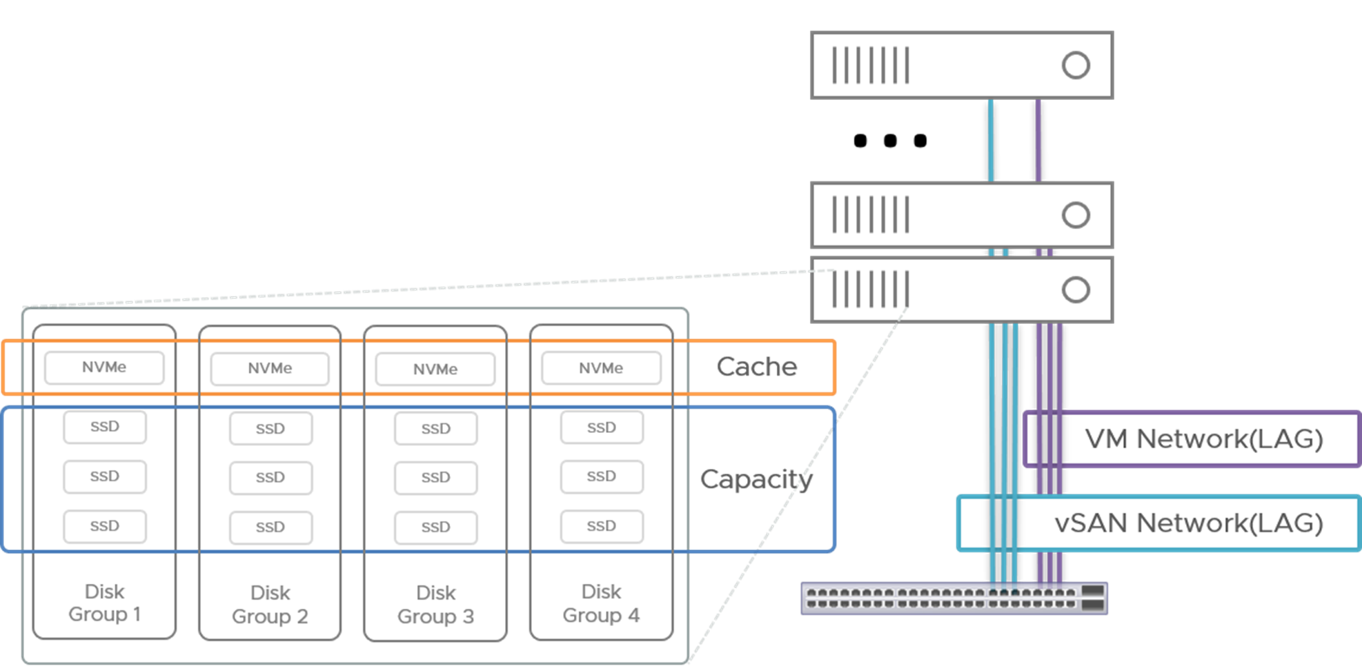
Figure 2. Disk Group Configuration
Storage Policy
Two different vSAN storage policies were created:
- FTT=0 (no additional replica) with data locality or Host Affinity enabled
- FTT= 1 (1 additional replica per object) with no Host Affinity
The stripe width (SW) was set to 12 (equal to the number of capacity disks per host). It is highly advised to use a stripe width that is optimized for number of capacity disks in a vSAN node.
In both test cases (FTT=0 and FTT=1), all VM disks (VMDKs) were created with that type of storage policy. One 100GB VMDK was created on each VM for that VM’s operating system. Additionally, the primary VMs received one additional 100GB VMDK while the worker VMs received six additional VMDKs, 700 GB each for FTT=0 and half that size, 350 GB for the redundant FTT=1.
VMs and VMDK
Two VMs were installed on each server. Setting the number of vCPUs equal to the number of physical cores (32) provides the best performance for vSAN. The 32 vCPUs were evenly distributed to the VMs, 16 each. For vSAN, we left 20% of the server memory for ESXi (see KB2113954 for the minimum memory requirement of vSAN), so the remaining 400 GiB was divided equally between the two VMs. On all VMs, the virtual NIC connected to the inter-VM VMware vSphere Distributed Switch™ was assigned an IP address internal to the cluster. The vmxnet3 driver was used for all network connections. Each virtual machine was installed with the CentOS 7.5 operating system (https://www.centos.org/download), which includes the latest Spectre/Meltdown patches.
- The OS disk was placed on a dedicated PVSCSI controller and the data disks were spread evenly over other three PVSCSI controllers.
- The six VMDKs on each worker VM were formatted using the ext4 filesystem, and the resulting data disks were used to create the Hadoop filesystem. Given the non-redundant character of FTT=0, the Hadoop cluster with that storage policy had roughly twice the raw HFDS capacity than that of FTT=1, 47.73 TB vs. 23.51TB. However, since vSAN with FTT=1 provides data block redundancy, the HDFS block redundancy (dfs.replication) was reduced from the default 3 to 2 for the FTT=1 tests. Therefore, the final available HDFS file size with the two policies was in the ratio of 1.5:1 (15.91 TB for FTT=0 and 11.76 TB for FTT=1).
Table 3 lists the vSAN storage configuration parameters.
Table 3. vSAN Storage Configurations
| Feature |
FTT=0, Host Affinity |
FTT=1, No Host Affinity |
|---|---|---|
| Data locality |
Host Local |
None |
| Data VMDKs per worker VM |
6x 700 GB |
6x 350 GB |
| vSAN storage used/capacity |
52.65 / 69.86 TB |
53.88 / 69.86 TB |
| Stripe width |
12 |
12 |
| vSAN replication factor |
1 |
2 |
| HDFS configured capacity |
47.73 TB |
23.51 TB |
| Default HDFS replication factor |
3 |
2 |
| HDFS Max file size at default replication factor |
15.91 TB |
11.76 TB |
Apache Hadoop/Spark Configuration
As shown in Table 4, there are three types of servers or nodes in a Hadoop cluster:
- Gateway/Edge server: One or more gateway servers act as client systems for Hadoop applications and provide a remote access point for users of cluster applications.
- Master server: Run the Hadoop master services such as the HDFS NameNode and the Yet Another Resource Negotiator (YARN) ResourceManager and their associated services (JobHistory Server, for example), as well as other Hadoop services such as Hive, Oozie, and Hue.
- Worker server: Only run the resource-intensive HDFS DataNode role and the YARN NodeManager role (which also serve as Spark executors).
Table 4. Hadoop VM Configurations
|
GATEWAY/edge VM |
Master VM |
Worker VM |
|
|---|---|---|---|
| Quantity |
1 |
2 |
12 |
| vCPU |
16 |
||
| Memory |
200 GiB |
||
| OS VMDK size |
250 GB |
100 GB |
100 GB |
| Data Disks |
1x 100 GB |
1x 100 GB |
6x 350(FTT=1)/700(FTT=0) GB |
| Roles | Cloudera Manager, ZooKeeper Server, HDFS JournalNode, HDFS gateway, YARN gateway, Hive gateway, Spark gateway, Spark History Server, Hive Metastore Server, Hive Server2, Hive WebHCat Server, Hue Server, Oozie Server | HDFS NameNode (active/standby), YARN ResourceManager (standby/primary), ZooKeeper Server, HDFS JournalNode, HDFS Balancer, HDFS FailoverController, HDFS HttpFS, HDFS NFS gateway | HDFS DataNode, YARN NodeManager, Spark Executor |
Figure 3 shows the cluster infrastructure. For the Hadoop tests, two of the servers ran infrastructure VMs to manage the Hadoop cluster. On the first infrastructure server, a VM hosted the gateway node, running the Cloudera Manager and several other Hadoop functions as well as the gateways for the HDFS, YARN, Spark, and Hive services. These two infrastructure servers each hosted a primary VM, on which the active and passive NameNode and ResourceManager components and associated services ran. The active NameNode and active ResourceManager ran on different servers for best distribution of the CPU load, with the standby of each on the opposite primary node. This also guarantees the highest cluster availability. For NameNode and ResourceManager high availability, at least three ZooKeeper services and three HDFS JournalNodes are required. Two of the ZooKeeper and Journal Node services ran on the two infrastructure servers; the third set ran on the first worker node.
The other six servers, the worker servers, hosted two VMs each, running only the worker services, HDFS DataNode, and YARN NodeManager. Spark executors ran on the YARN NodeManagers. As noted above, one worker VM also ran a ZooKeeper and Journal Node service. With the very small CPU/memory overhead, these processes do not measurably impact the worker services. However, for larger deployments with other roles running on the infrastructure VMs, it might be necessary to run three infrastructure servers, in which case the third ZooKeeper and Journal Nodes may be run on one of the infrastructure servers.
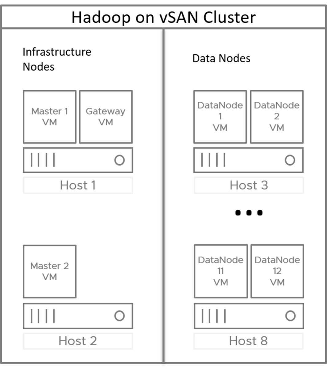
Figure 3. Big Data Cluster—Infrastructure and Worker Nodes
The components of Hadoop used in these tests were HDFS, YARN, and ZooKeeper, with roles deployed as shown in Table 4. Spark was installed on YARN, which means the Spark executors ran in YARN containers.
Hadoop Virtualization Extensions (HVE), an open source Hadoop add-on (https://issues.apache.org/jira/browse/HADOOP-8468) was employed to prevent multiple copies of a given HDFS block from being placed on the same physical server for availability reasons. HVE adds an additional layer to the HDFS rack awareness, node group, to enable the user to identify which VMs reside on the same physical server. HDFS uses that information in its block placement strategy.
In Hadoop tuning, the two key cluster parameters that need to be set are yarn.nodemanager.resource.cpu-vcores and yarn.nodemanager.resource.memory-mb, which tell YARN how much CPU and memory resources, respectively, can be allocated to task containers in each worker node.
For CPU resources, the vCPUs in each worker VM were exactly committed to YARN containers, that is, yarn.nodemanager.resource.cpu-vcores was set equal to the number of vCPUs in each VM, 16. For memory, about 40 GiB of the VM’s 200 GiB needs to be set aside for the operating system and the JVMs running the DataNode and NodeManager processes, leaving 160 GiB for yarn.nodemanager.resource.memory-mb. Thus, for the 12 worker nodes, the total vcores available was 192 and the total memory was 1,920 GiB.
A few additional parameters were changed from their default value. The buffer space allocated on each mapper to contain the input split while being processed (mapreduce.task.io.sort.mb) was raised to its maximum value, 2,047 MiB (about 2 GiB) to accommodate the very large block size that was used in the TeraSort suite (in Table 5). The amount of memory dedicated to the Application Master process, yarn.app.mapreduce.am.resource.mb, was raised from 1 GiB to 4 GiB. The parameter yarn.scheduler.increment-allocation-mb was lowered from 512 MiB to 256 MiB to allow finer grained specification of task sizes. The log levels of all key processes were turned down from the default of INFO to WARN for the production use, but the much lower levels of log writes did not have a measurable impact on application performance.
These global parameters are summarized in Table 5.
Table 5. Key Hadoop/Spark Cluster Parameters Used in Tests
| PARAMETER |
DEFAULT |
CONFIGURED |
|---|---|---|
| yarn.nodemanager.resource.cpu-vcores |
- |
16 |
| yarn.nodemanager.resource.memory-mb |
- |
160 GiB |
| mapreduce.task.io.sort.mb |
256 MiB |
2047 MiB |
| yarn.app.mapreduce.am.resource.mb |
1 GiB |
4 GiB |
| yarn.scheduler.increment-allocation-mb |
512 MiB |
256 MiB |
| Log Level on HDFS, YARN, Hive |
INFO |
WARN |
| Note: MiB = 2**20 (1048576) bytes, GiB = 2**30 (1073741824) bytes | ||
See more details about the general Hadoop/YARN tuning in FAST Virtualized Hadoop and Spark on All-Flash Disks.
Hadoop Cluster Scaling
Hadoop and Spark are extremely scalable, meaning the performance will increase almost linearly with the number of worker servers. The configuration used in this test is sufficient for an 8-server cluster. For larger clusters up to 16 servers, all the additional servers should be added as worker servers. For larger clusters with more than 16 servers, a third server should be dedicated to VMs running the Hadoop primary processes. The Hadoop performance scales linearly with the increase of worker nodes as shown in Table 6.
Table 6. Hadoop Cluster Scaling
|
Cluster SIZE # of Servers |
# of Servers Dedicated to Primary VMs |
# of Servers Dedicated to Worker VMs |
# of Worker VMs |
Expected Performance Scaling |
Total vSAN Storage |
|---|---|---|---|---|---|
|
8 |
2 |
6 |
12 |
1x |
70 TB |
|
16 |
2 |
14 |
28 |
2.3x |
140 TB |
|
32 |
3 |
29 |
58 |
4.8x |
280 TB |
|
48 |
3 |
45 |
90 |
7.5x |
420 TB |
Workloads
The benchmarks used in the solution are: - Cloudera storage validation - Hadoop MapReduce - Spark
Overview
We used several standard benchmarks that exercise the key components of a Big Data cluster in this solution test. These benchmarks may be used by customers as a starting point for characterizing their Big Data clusters, but their own applications will provide the best guidance for choosing the correct architecture. The benchmarks used in the solution are:
- Cloudera storage validation
- Hadoop MapReduce
- TeraSort Suite
- TestDFSIO
- Spark
- K-means clustering
- Logistic regression classification
- Random forest decision trees
- IoT analytics benchmark
Cloudera Storage Validation
Cloudera provides storage performance KPIs as the prerequisite of running CDH on a given system. Also, Cloudera provides a tool-kit to conduct a series of performance tests including a microbenchmark, HBase, and Kudu. See the Cloudera Enterprise Storage Device Acceptance Criteria Guide for detailed information.
Hadoop MapReduce
Two industry-standard MapReduce benchmarks, the TeraSort suite and TestDFSIO, were used for measuring the cluster performance.
TeraSort Suite
The TeraSort suite (TeraGen/TeraSort/TeraValidate) is the most commonly used Hadoop benchmark and ships with all Hadoop distributions. By first creating a large dataset, then sorting it, and finally validating that the sort was correct, the suite exercises many of Hadoop’s functions and stresses CPU, memory, disk, and network.
TeraGen generates a specified number of 100 byte records, each with a randomized key occupying the first 10 bytes, creating the default number of replicas as set by dfs.replication. In these tests 10 and 30 billion records were specified resulting in datasets of 1 and 3 TB. TeraSort sorts the TeraGen output, creating one replica of the sorted output. In the first phase of TeraSort, the map tasks read the dataset from HDFS. Following that is a CPU-intensive phase where map tasks partition the records they have processed by a computed key range, sort them by key, and spill them to disk. At this point, the reduce tasks take over, fetch the files from each mapper corresponding to the keys associated with that reducer, and then merge the files for each key (sorting them in the process) with several passes, and finally write to disk. TeraValidate, which validates that the TeraSort output is indeed in sorted order, is mainly a read operation with a single reduce task at the end.
TeraGen is a large block, sequential write-heavy workload, with a block size of 512KB. TeraSort starts with reads as the dataset is read from HDFS, then moves to a read/write mix as data is shuffled between task during the sort, and then concludes with a short write-dominated phase as the sorted data is written to HDFS. TeraValidate is a brief read-only phase.
TestDFSIO
TestDFSIO is a write-intensive HDFS stress tool also supplied with every distribution. It generates a specified number of files of a specified size. In these tests 1,000 files of size 1 GB, 3 GB, or 10 GB files were created for total size of 1, 3, and 10 TB. Like TeraGen, the I/O pattern is large block (512KB) sequential writes.
Spark
Three standard analytic programs from the Spark machine learning library (MLlib), K-means clustering, Logistic Regression classification, and Random Forest decision trees, were driven using spark-perf (Databricks, 2015). In addition, a new, VMware-developed benchmark, IoT Analytics Benchmark, which models real-time machine learning on Internet-of-Things data streams, was used in the comparison. The benchmark is available from Github.
All of the Spark workloads ran mainly in memory and thus did not see much performance difference between FTT=0 with Host Affinity and FTT=1 without Host Affinity.
K-means Clustering
Clustering is used for analytic tasks such as customer segmentation for purposes of ad placement or product recommendations. K-means groups input into a specified number, k, of clusters in a multi-dimensional space. The code tested groups a large training set into the specified number of clusters and uses this to build a model to quickly place a real input set into one of the groups.
Two K-means tests were run, each with 5 million examples. The number of groups was set to 20 in each. The number of features was varied, with 5,750 and 11,500 features generating dataset sizes of 500 GB and 1 TB. The training time reported by the benchmark kit was recorded. Four runs at each size were performed, with the first one being discarded and the remaining three averaged to give the reported elapsed time.
Logistic Regression Classification
Logistic regression (LR) is a binary classifier used in tools such as credit card fraud detection and spam filters. Given a training set of credit card transaction examples with, say, 20 features, (date, time, location, credit card number, amount, etc.) and whether that example is valid or not, LR builds a numerical model that is used to quickly determine if subsequent (real) transactions are fraudulent.
Three LR tests were run, each with 5 million examples. The number of groups was set to 20 in each. The number of features was varied, with 5,750 and 11,500 features generating dataset sizes of 500 GB and 1 TB. The training time reported by the benchmark kit was recorded. Four runs at each size were performed, with the first one being discarded and the remaining three averaged to give the reported elapsed time.
Random Forest Decision Trees
Random Forest automates any kind of decision making or classification algorithm by first creating a model with a set of training data, with the outcomes included. Random Forest runs an ensemble of decision trees in order to reduce the risk of overfitting the training data.
Three Random Forest tests were run, each with 5 million examples. The number of trees was set to 10 in each. The number of features was varied with 7,500 and 15,000 features generating dataset sizes of 500GB and 1 TB. The training time reported by the benchmark kit was recorded. Four runs at each size were performed, with the first one discarded and the remaining three averaged to give the reported elapsed time.
The Spark MLlib code enables the specification of the number of partitions that each Spark resilient distributed dataset (RDD) employs. For these tests, the number of partitions was initially set equal to the number of Spark executors times the number of cores in each but was increased in certain configurations as necessary.
IoT Analytics Benchmark
The IoT Analytics Benchmark is a simulation of data analytics being run on a stream of sensor data, for example, factory machines being monitored for impending failure conditions.
The IoT Analytics Benchmark consists of three Spark programs:
- iotgen generates synthetic training data files using a simple randomized model. Each row of sensor values is preceded by a label, either 1, or 0, indicating whether that set of values would trigger the failure condition
- iottrain uses the pre-labeled training data to train a Spark machine learning library model using logistic regression
- iotstream applies that model to a stream of incoming sensor values using Spark Streaming, indicating when the impending failure conditions need attention.
In the solution tests, we used iottrain to generate datasets of 500 GB and 750 GB, and then iottrain ran against these datasets to train the machine learning models used by iotstream.
In each case, we ran four tests with the first one discarded, and the last three averaged for the reported results.
Performance Testing and Results
We performed the following tests based on different workload benchmarks: - Cloudera storage validation - TeraSort testing - TestDFSIO testing - Spark testing - IoT Analytics testing
Cloudera Storage Validation Results
All the KPIs mentioned in the Cloudera Enterprise Storage Device Acceptance Criteria Guide were met.
TeraSort Results
The commands to run the three components of the TeraSort suite (TeraGen, TeraSort, and TeraValidate) are shown in appendix. The dfs.blocksize was set at 1 GiB to take advantage of the large memory available to YARN, and mapreduce.task.io.sort.mb was consequently set to the largest possible value, 2,047 MiB, to minimize spills to disk during the map processing of each HDFS block.
It was found experimentally that the map and the reduce tasks for all components ran faster with 1 vcore assigned to each. With 192 total cores available on the cluster, 192 1-vcore tasks could run simultaneously. However, a vcore must be set aside to run the ApplicationMaster, leaving 191 tasks. With this number of tasks, each task container can be assigned 10 GB of the total 1,920 GB in the cluster.
The TeraSort results are shown in Table 7 and Table 8 and plotted in Figure 4. The write-intensive TeraGen components are about 50% faster using the FTT=0 with Host Affinity storage policy due to the data locality and less number of copy per object while TeraSort, a mix of I/O and compute, runs about 20% faster. TeraValidate, a short, read-intensive workload, is about even.
- For FTT=0, the maximum write bandwidth to the vSAN datastore was about 2.6 GB/s for each of the 6 hosts serving as worker servers, for a total of about 16 GB/s, with the peak IOPS around 5,000 per server and latencies of about 450 ms.
- For FTT=1, the maximum write bandwidth was about 1.1 GB/s, for a total of about 6.6 GB/s, with the peak IOPS around 2,800 per server and latencies of about 1,100 ms.
Table 7. TeraSort Performance Results—1 TB (Smaller is Better)
| vSAN Storage Policy | TERAGEN ELAPSED TIME (SEC) | TERASORT ELAPSED TIME (SEC) | TERAVALIDATE ELAPSED TIME (SEC) |
|---|---|---|---|
| FTT=0, Host Affinity | 211.4 | 514.6 | 76.9 |
| FTT=1, No Host Affinity | 326.4 | 620.5 | 77.2 |
| Performance advantage, FTT=0 over FTT=1 | 54.4% | 20.6% | 0.4% |
Table 8. TeraSort Performance Results—3 TB (Smaller is Better)
| vSAN Storage Policy | TERAGEN ELAPSED TIME (SEC) | TERASORT ELAPSED TIME (SEC) | TERAVALIDATE ELAPSED TIME (SEC) |
|---|---|---|---|
| FTT=0, Host Affinity | 648.6 | 1705.5 | 227.2 |
| FTT=1, No Host Affinity | 1016.2 | 2106.0 | 318.7 |
| Performance advantage, FTT=0 over FTT=1 | 56.7% | 23.3% | 40.3% |

Figure 4. TeraSort Suite Performance Showing FTT=0 vs. FTT=1
TestDFSIO Results
TestDFSIO was run as shown in Table 9 to generate the output of 1, 3, and 10 TB by writing 1,000 files of increasing size. As in TeraSort, the number of vcores and memory size per map task was adjusted experimentally for best performance. For the write-intensive map phase, 191 maps with 1 vcore and 10 GiB each were used. There is a short reduce phase at the end of the test which was found to run best with 2 cores per reduce task.
The results are shown in Table 9 and Figure 5. Like TeraGen, TestDFSIO benefits from the data locality of the FTT=0 configuration, with performance improvements of 40% or more over FTT=1.
Table 9. TestDFSIO Performance Results (Smaller is Better)
| vSAN Storage Policy | 1TB TestDFSIO ELAPSED TIME (SEC) | 3TB TestDFSIO ELAPSED TIME (SEC) | 10TB TestDFSIO ELAPSED TIME (SEC) |
|---|---|---|---|
| FTT=0, Host Affinity | 243.6 | 664.2 | 2437.1 |
| FTT=1, No Host Affinity | 354.4 | 1006.1 | 4173.1 |
| Performance advantage, FTT=0 over FTT=1 | 41.8% | 51.5% | 71.2% |

Figure 5. TestDFSIO Performance
Spark Results
The three Spark MLlib benchmarks were controlled by configuration files exposing many Spark and algorithm parameters. A few parameters were modified from their default values. From experimentation, it was found that the three programs ran fastest with 2 vcores and 20 GiB per each of 95 executors, using up most of the 192 vcores and 1,920 GiB available in the cluster. The 20 GiB was specified as 16 GiB spark.executor.memory plus 4 GiB spark.yarn.executor.memoryOverhead. The number of resilient distributed dataset (RDD) partitions was set to the number of executors times the number of cores per executor, or 190, so there would be one partition per core. 20 GiB was assigned to the Spark driver process (spark.driver.memory).
All three MLlib applications were tested with training dataset sizes of 500 GB and 1 TB. The cluster memory was sufficient to contain all datasets. For each test, first a training set of the specified size was created. Then the machine learning component was executed and timed, with the training set ingested and used to build the mathematical model to be used to classify real input data. The training times of four runs were recorded, with the first one discarded and the average of the remaining three values reported here. Table 10 lists the complete Spark MLlib test parameters.
Table 10. Spark Machine Learning Program Parameters
|
Parameter |
k-Means |
Logistic Regression |
Random Forest |
|---|---|---|---|
| # examples |
5,000,000 |
5,000,000 |
5,000,000 |
| 500 GB # features |
5,750 |
5,750 |
7,500 |
| 1 TB # features |
11,500 |
11,500 |
15,000 |
| # executors |
95 |
95 |
95 |
| Cores per executor |
2 |
2 |
2 |
| 500 GB # partitions |
190 |
190 |
190 |
| 1 TB # partitions |
190 |
190 |
190 |
| Spark driver memory |
20 GiB |
20 GiB |
20 GiB |
| Executor memory |
16 GiB |
16 GiB |
16 GiB |
| Executor overhead memory |
4 GiB |
4 GiB |
4 GiB |
The Spark Machine Learning test results are shown from Table 11 to Table 13 and plotted in Figure 5. Since these programs execute mainly in memory, there is very little (about 5% or less) performance difference between FTT=0 and FTT=1.
Table 11. Spark k-Means Performance Results—Smaller is Better
|
vSAN Storage Policy |
500 GB K-Means ELAPSED TIME (SEC) |
1 TB k-Means ELAPSED TIME (SEC) |
|
FTT=0, Host Affinity |
74.8 |
158.6 |
|
FTT=1, No Host Affinity |
78.7 |
167.1 |
|
Performance advantage, FTT=0 over FTT=1 |
5.2% |
5.4% |
Table 12. Spark Logistic Regression Performance Results—Smaller is Better
|
vSAN Storage Policy |
500 GB Logistic Regression ELAPSED TIME (SEC) |
1 TB Logistic Regression ELAPSED TIME (SEC) |
|
FTT=0, Host Affinity |
21.9 |
36.7 |
|
FTT=1, No Host Affinity |
22.3 |
36.8 |
|
Performance advantage, FTT=0 over FTT=1 |
1.8% |
0.2% |
Table 13. Spark Random Forest Performance Results—Smaller is Better
|
VSAN STORAGE POLICY |
500 GB RANDOM FOREST ELAPSED TIME (SEC) |
1 TB RANDOM FOREST ELAPSED TIME (SEC) |
|
FTT=0, Host Affinity |
125.7 |
227.3 |
|
FTT=1, No Host Affinity |
124.2 |
219.7 |
|
Performance advantage, FTT=0 over FTT=1 |
-1.2% |
-3.4% |

Figure 6. Spark K-means Performance
IoT Analytics Results
The IoT Analytics Benchmark parameters are fully documented in the benchmark’s Github site. As shown in Table 15, the programs were run using the standard spark-submit command, with Spark parameters immediately following, and the specific benchmark parameters at the end.
Single vcore executors are optimum for the write-based data generation (iotgen) program. As with TeraSort, 191 such executors were run (leaving 1 container available to YARN for the Application Master), each using a total of 10 GiB (8 GiB executor memory plus 2GiB overhead). The parameters following iotstream_2.10-0.0.1.jar specify the number of rows, sensors per row, and partitions, and then the storage protocol, folder and file name of the output file. The final parameter (25215000) was used to control the percentage of rows that were coded to be “True” for model training.
For the model training (iottrain) program, 4 cores per executor were found to be optimal. Thus, 47 such executors were run (consuming a total of 188 vcores) each using a total of 40 GiB (32 GiB executor memory plus 8 GiB overhead). The parameters following iotstream_2.10-0.0.1.jar specify the storage protocol, folder and file name of the training data file and the name of the output file containing the trained model.
Table 14, Table 15, and Figure 7 show the IoT Analytics Benchmark performance results. As with the other Spark workloads, both the data generation and model training components fit mainly in memory so there was very little difference (2% or less) between the performance of the FTT=0 with Host Affinity configuration and the FTT=1 configuration.
Table 14. IoT Analytics Benchmark Data Generation Performance Results—Smaller is Better
|
VSAN STORAGE POLICY |
500 GB IOTGEN ELAPSED TIME (SEC) |
750 GB IOTGEN ELAPSED TIME (SEC) |
|
FTT=0, Host Affinity |
734.5 |
1117.1 |
|
FTT=1, No Host Affinity |
728.3 |
1095.2 |
|
Performance advantage, FTT=0 over FTT=1 |
-0.8% |
-2.0% |
Table 15. IOT Analytics Benchmark Model Training Performance Results—Smaller is Better
|
VSAN STORAGE POLICY |
500 GB IOTTRAIN ELAPSED TIME (SEC) |
750 GB IOTRAIN ELAPSED TIME (SEC) |
|
FTT=0, Host Affinity |
303.7 |
473.9 |
|
FTT=1, No Host Affinity |
305.3 |
469.1 |
|
Performance advantage, FTT=0 over FTT=1 |
0.5% |
-1.0% |

Figure 7. IoT Analytics Benchmark Results
Failover Testing
In the failover testing, we performed the host and disk failure tests with the FTT=1 setting and the FTT=0 with Host Affinity setting
Host Failure
With the FTT=0 configuration, each VM or VMDK has only one copy in the cluster. To ensure that VMs can access the data from the local host, vSAN 6.7 introduced the Host Affinity rule option for the vSAN storage policy. With Host Affinity that copy is stored on the same host where the VM is located.
However, with the FTT=0 and Host Affinity feature configured, Hadoop needs to handle the failure scenario. By setting HDFS redundancy number to 3 and having HVE properly configured to prevent multiple copies of a given HDFS block from being placed on the same physical server, the Hadoop cluster can tolerate up to two physical hosts failure without requiring re-ingestion of data.
We set FTT=0 and conducted a TeraSort suite 3TB test and powered off one physical host when TeraGen was 60% completed, to validate the data availability upon host failure. The test completed without any availability impact.
Similarly, we repeated the same steps on the FTT=1 configuration, the TeraSort Suite test also completed without any data availability impact.
Disk Failure
When the Hadoop cluster is configured with FTT=0 and Host Affinity, any vSAN capacity or cache disk failure might cause the VMs on that host to become inaccessible, which would have the same impact as the host failure scenario.
When the Hadoop cluster is configured with FTT=1, the TeraSort Suite took the same time to complete as the test with no failure scenario.
FTT=1 and FTT=0 with Host Affinity Considerations and Comparison
This section lists the considerations and comparison results of these two configurations from the network, capacity, performance, and availability perspectives.
Network Configuration
There is very little vSAN network traffic on FTT=0 with Host Affinity; therefore, if there are only two 10GbE network interface ports, we can trunk the ports as Linked Aggregated Group and share the uplink between vSAN VMkernel and VM network.
With the FTT=1 configuration, to prevent the traffic competition between VM network traffic and vSAN network traffic, we recommend physically separating the VM network and vSAN VMkernel by assigning a single 10GbE port as active and use the other port as standby in a reversed order, which is illustrated in Figure 8. In this case, the bandwidth of both VM network traffic and vSAN network traffic is limited to 10Gb.

Figure 8. Networking Design of FTT=1 Configuration with two 10 GbE NICs
Capacity
Unlike FTT=0, for FTT=1, there is an additional copy of each VMDK, so the HDFS capacity with FTT=0 configuration is about two times that of the FTT=1. By setting the HDFS replication factor to 3 for FTT=0 and 2 for FTT=1, the HDFS maximum files size ratio between FTT=0 and FTT=1 is about 4:3.
Performance
For I/O intensive workloads such as TeraSort Suite and TestDFSIO, Host Affinity significantly improves time to completion, this is primarily because of the reduced I/O amplification attributed to running vSAN without any replication.
Availability and Maintenance
With FTT=0 and Host Affinity configured, the HDFS redundancy factor was set to 3, which meant the Hadoop cluster could tolerate up to two physical hosts failure.
With FTT=1, the HDFS redundancy factor was set to 2 to prevent application failure, even in total there are four copies for each block (two copies on the HDFS layer and two copies on the vSAN layer), the Hadoop cluster can only tolerate one host failure because two HDFS replicas might be placed on the same physical host on the vSAN layer.
Host Failure Scenario
With host affinity, host failure would require the VMs to be manually recreated, all the impacted VMs should be deployed on the same physical host to maintain the consistency with rack awareness data shared with the application.
However, with the FTT=1 configuration, all the VMs will be migrated and preserved on other hosts by vSphere HA, hence no VMs need to be rebuilt after the failed host is recovered.
Disk Failure Scenario
When the capacity or cache disk failure happened to the vSAN cluster with FTT=0 and Host Affinity configured, we still need to rebuild the DataNode or Master VMs on the replacement host because with the stripe width set to 12, there is high probability that both VMs will become inaccessible due to the disk failure. And the performance impact is the same as the host failure.
If the disk failure occurs on FTT=1 configuration, there is no VM loss or failure, all the VMs will be still up and running. We just need to replace the failed disk and rebuild the failed vSAN disk group if necessary without rebuilding any Hadoop components, vSAN would do a partial rebuild of the failed components completely transparent to Hadoop.
Table 16. Comparison between FTT=1 and FTT=0 with Host Affinity
|
CONSIDERATIONS |
FTT=0 WITH HOST AFFINITY |
FTT=1 |
|
HDFS capacity |
More |
Less |
|
I/O performance |
Better |
Good |
|
Host failure tolerance |
2 (with RF set to 3) |
1 (with RF set to 2) |
|
Performance impact of host failure |
No data loss; some performance degradation |
|
|
Rebuild VMs when failed host coming back |
Yes |
No |
|
Data rebuild impact at application layer with disk failure |
Same as the host failure |
None |
Solution Summary
As the adoption of both big data and HCI continues at a rapid pace, VMware vSAN provides the simplicity, agility, and manageability to deploy and configure the next-generation applications.
This solution provides alternatives to deploy your next-generation applications on vSAN, you can adopt the FTT=1 configuration if you want to leverage vSphere HA to reduce the operational cost when the failure happens; if you want extra performance, capacity or availability, you can use FTT=0 with Host Affinity configuration as an approach.
Appendix: Testing Commands
TeraSort Suite Performance Test Commands
TeraGen-1TB:
time hadoop jar <path>/hadoop-mapreduce-examples.jar teragen -Ddfs.blocksize=1342177280 -Dmapreduce.job.maps=191 -Dmapreduce.map.memory.mb=10240 -Dmapreduce.map.cpu.vcores=1 10000000000 terasort1TB_input
TeraSort-1TB:
time hadoop jar <path>/hadoop-mapreduce-examples.jar terasort -Ddfs.blocksize=1342177280 -Dmapreduce.job.reduces=191 -Dmapreduce.map.memory.mb=10240 -Dmapreduce.reduce.memory.mb=10240 -Dmapreduce.map.cpu.vcores=1 -Dmapreduce.reduce.cpu.vcores=1 terasort1TB_input terasort1TB_output
TeraValidate-1TB:
time hadoop jar <path>/hadoop-mapreduce-examples.jar teravalidate -Dmapreduce.map.memory.mb=10240 terasort1TB_output terasort1TB_validate
TeraGen-3TB:
time hadoop jar <path>/hadoop-mapreduce-examples.jar teragen -Ddfs.blocksize=1342177280 -Dmapreduce.job.maps=191 -Dmapreduce.map.memory.mb=10240 -Dmapreduce.map.cpu.vcores=1 30000000000 terasort3TB_input
TeraSort-3TB:
time hadoop jar <path>/hadoop-mapreduce-examples.jar terasort -Ddfs.blocksize=1342177280 -Dmapreduce.job.reduces=191 -Dmapreduce.map.memory.mb=10240 -Dmapreduce.reduce.memory.mb=10240 -Dmapreduce.map.cpu.vcores=1 -Dmapreduce.reduce.cpu.vcores=1 terasort3TB_input terasort3TB_output
TeraValidate-3TB:
time hadoop jar <path>/hadoop-mapreduce-examples.jar teravalidate -Dmapreduce.map.memory.mb=10240 terasort3TB_output terasort3TB_validate
TestDFSIO Test Commands
hadoop jar <path>/TestDFSIO -Ddfs.blocksize=1342177280 -Dmapreduce.map.memory.mb=10240 -Dmapreduce.reduce.cpu.vcores=2 -write -nrFiles 1000 -size 1GB/3GB/10GB
IoT Analytics Benchmark Commands
500 GB Data Generation:
spark-submit --num-executors 191 --executor-cores 1 --executor-memory 8g --conf spark.yarn.executor.memoryOverhead=2048 --name iotgen_lr --class com.iotstream.iotgen_lr iotstream_2.10-0.0.1.jar 6713459 10000 191 HDFS sd sensor_data6713459_10000_10_191_1 25215000
750 GB Data Generation:
spark-submit --num-executors 191 --executor-cores 1 --executor-memory 8g --conf spark.yarn.executor.memoryOverhead=2048 --name iotgen_lr --class com.iotstream.iotgen_lr iotstream_2.10-0.0.1.jar 10070475 10000 191 HDFS sd sensor_data10070475_10000_10_191_1 25215000
500 GB Model Training:
spark-submit --num-executors 47 --executor-cores 4 --executor-memory 32g --conf spark.yarn.executor.memoryOverhead=8192 --name iottrain_lr --class com.iotstream.iottrain_lr iotstream_2.10-0.0.1.jar HDFS sd sensor_data6713459_10000_10_191_1 lr10K_2
750 GB Model Training:
spark-submit --num-executors 47 --executor-cores 4 --executor-memory 32g --conf spark.yarn.executor.memoryOverhead=8192 --name iottrain_lr --class com.iotstream.iottrain_lr iotstream_2.10-0.0.1.jar HDFS sd sensor_data10070475_10000_10_191_1 lr10K_3
References
The following documents are the reference for this solution:
- VMware Product Documentation:
- Cloudera/Hadoop Reference Documentation:
- Other Reference:
About the Authors
Four co-authors wrote the original version of this paper:
- Dave Jaffe, Staff Engineer specializing in Big Data Performance in the Performance Engineering team in VMware
- Chen Wei, Senior Solution Architect in the Product Enablement team of the Storage and Availability Business Unit in VMware
- Sumit Lahiri, Product Line Manager for vSAN software platform in the Storage and Availability Business Unit in VMware
- Dwai Lahiri, Senior Solutions Architect in Cloudera’s Partner Engineering team
Catherine Xu, Senior Technical Writer in the Product Enablement team of the Storage and Availability Business Unit, edited this paper to ensure that the contents conform to the VMware writing style.