
Troubleshooting vSAN Performance
Executive Summary
An infrastructure that delivers sufficient performance for applications is a table stake for data center administrators. The lack of sufficient and predictable performance can not only impact the VMs that run in an environment, but the consumers who use those applications. Determining the root cause of performance issues in any environment can be a challenge, but with environments running dozens, if not hundreds of virtual workloads, pinpointing the exact causes, and understanding the options for mitigation can be difficult for even the experienced administrator.
VMware vSAN is a distributed storage solution that is fully integrated into VMware vSphere. By aggregating local storage devices in each host across a cluster, vSAN is a unique, and innovative approach to providing cluster-wide, shared storage and data services to all virtual workloads running in a cluster. While it eliminates many of the design, operation and performance challenges associated with three-tier architectures using storage arrays, it introduces additional considerations in diagnosing and mitigating performance issues that may be storage related.
This document will help the reader better understand how to identify, quantify, and remediate performance issues of real workloads running in a vSAN powered environment running all-flash. It is not a step-by-step guide for all possible situations, but rather, a framework of considerations in how to address problems that are perceived to be performance related. The example provided in Appendix C will illustrate how this framework can be used. The information provided assumes an understanding of virtualization, vSAN, infrastructures, and applications.
Diagnostics and Remediation Overview
vSAN environments may experience performance challenges in a variety of circumstances. This includes:
- Proof of Concept (PoC) phase using synthetic testing, or performance benchmarking
- Initial migration of production workloads to vSAN
- Normal day-to-day operation of production workloads
- Evolving demands of production workloads
The primary area of focus of this document is related to production workloads in a vSAN environment. Many of the same mitigation steps can be used to evaluate performance challenges when using synthetic I/O testing during an initial PoC. The performance evaluation checklists found in the vSAN Proof of Concept Guides offers a collection of guidance and practices for PoCs that will be helpful for customers in that phase of the process. Accurately diagnosing performance issues of a production environment requires care, persistence and correctly understanding the factors that can commonly contribute to performance challenges.
Contributing Factors
Several factors influence the expected outcome of system performance in a customer’s environment, and the behavior of workloads for that specific organization. Most fall in one of the five categories, but are not mutually exclusive. These factors contribute to the performance vSAN is able to provide, as well as the performance perceived by users and administrators. When reviewing previous performance issues in any architecture where a root cause was determined, you'll find that the reason can often trace back to one or more of these five categories.

Figure 1. Important factors that contribute to performance expectations and outcomes
Understanding the contributing factors to a performance issue is critical to knowing what information needs to be collected to begin the process of diagnosis and mitigation.
Process of Diagnosis and Mitigation
A process for diagnosis and mitigation helps work through the problem, and address it in a clear and systematic way. Without this level of discipline, further speculation and potential remedies to the issue will be scattered, and ineffective in addressing the actual issue. This process can be broken down into five steps:
- Identify and quantify. This step helps to clearly define the issue. Clarifying questions can help properly qualify the problem statement, which will allow for a more targeted approach to addressing. This process helps sort out real versus perceived issues, and focuses on the end result and supporting symptoms, without implying the cause of the issue.
- Discovery/Review - Environment. This step takes a review of the current configuration. This will help eliminate previously unnoticed basic configuration or topology issues that might be plaguing the environment.
- Discovery/Review - Workload. This step will help the reader review the applications and workflows. This will help a virtualization administrator better understand what the application is attempting to perform, and why.
- Performance Metrics - Insight. This step will review some of the key performance metrics to view, and how to interpret some of the findings the reader may see when observing their workloads. It clarifies what the performance metrics means, and how they relate to each other..
- Mitigation - Options in potential software and hardware changes. This step will help the reader step through the potential actions for mitigation.
A performance issue can be defined in a myriad of ways. For storage performance issues with production workloads, the primary indicator of storage performance challenges is I/O latency as seen by the guest VM running the application(s). Latency, and other critical metrics are discussed in greater detail in steps 4 and 5 of this diagnosis workflow. With guest VM latency being the leading symptom of insufficient performance of a production workload, and an understanding of the influencing factors that contribute to storage performance (shown in Figure 1.), the troubleshooting workflow for vSAN could be visualized similar to what is found in Figure 2.

Figure 2. A visual representation of a performance troubleshooting workflow for vSAN environments that represents the related factors
Notice the emphasis defining the issue, and the gathering of relevant information (Steps 2 & 3) about the environment. While it may be a bit time consuming, this one-time effort of information gathering is absolutely critical, as the information gathered will help identify potential bottlenecks, and suggest the most reasonable options for mitigating the issue. Most importantly, in reduces the chances of addressing the wrong item.
vSAN's distributed architecture means that sometimes traditional methods used for isolating the potential source of the issue needs to be altered. For example, isolating elements to a host is common practice in traditional, top-down approaches to troubleshooting. Those methods of isolation can be inherently more challenging with distributed storage as data may live across remote, and/or multiple hosts.
This document follows the process of diagnosis and mitigation described in Figure 2, and will elaborate on each step in an appropriate level of detail. Recommendations are provided on specific metrics to monitor (In Step 4, and Appendix A), and what they mean to the applications and the environment. Additionally, the reader will find a summary of useful tools (found In Appendix B) should there be a desire to explore the details at a deeper level. Troubleshooting performance issues can be difficult even under the best of circumstances. This is made worse by skipping valuable steps in gathering information about the issue to really understand and define the problem. Therefore, the information provided here places emphasis on understanding the environment and workloads over associating each potential performance problem with a single fix.
This document does not cover the details of how to evaluate vSAN for a PoC environment, nor does it provide detail on how to run synthetic I/O based performance benchmarks. The information provided here closely aligns with the recommendations found in the vSAN Proof of Concept Guides, which is a great resource to level-set an environment for performance evaluation.
Step #1: Identify and Quantify
Identifying the issue prior to taking any action
Properly identifying an issue is critical to timely resolution to an issue. Unlike break/fix issue where there is a clear delineation between functional and not functional, performance issues fall in an area more difficult to define and quantify. Perception can often play a part in this, which is why a measured approach should be taken in this initial phase of discovery. The following are questions that can be helpful in determining if there is a performance issue, the magnitude, and a bit of context around the reported problem.
Determine if there is a performance issue
- Source of the complaint? (Application owner? Application Consumer? DBA?, Infrastructure Admin? etc.)
- Is there verifiable data to support claim? (e.g. "before vs. after", captured environmental performance metrics, batch process completion times, comparison of performance with workload on vSAN vs other storage system, etc.)
Determine magnitude of performance issue
- What is the delta in performance? Rounding error, or significant? (Helps determine magnitude, and point to root cause)
- What is the percentage/frequency of the issue (quantifies how often/frequent it occurs. e.g. is performance poor, or mostly good, but inconsistent)
- Methods of measurement?
- What is being measured
- How is it being measured
- Where is it being measured
- Is it repeatable?
- Any notable events or changes since the performance degradation? Including, but not limited to:
- BIOS changes and updates
- NIC firmware updates
- New storage devices or other additions
- New switchgear
Determine if issue is beyond initial design scope
- How was success initially defined, and by whom?
- Did performance issue arise only after moving application/workload to vSAN?
- Did scope of cluster change?
- Additional workloads, and other demands?
- Scoped for affordability/density, but now concerned with performance?
- Additional data services enabled after initial deployment such as deduplication & compression, or data-at-rest encryption?
- Insufficient initial config? Was the initial BoM/spec of the cluster scoped for performance, or was it scoped for capacity/value?
- Was the performance testing recommendations found in the PoC guides followed prior to testing?
- Were synthetic tests (HCIBench) run prior to production to ensure base outcomes?
- What were the HCIBench test results prior to entering into production? Can they be referred to?
- What are the HCIBench test results currently?
Asking these very important questions also helps manage expectations on what the designed system is capable of performing. If a data center administrator was expecting their batch process completion time to be improved by 20%, and designed for that expectation, then that can be addressed. If one was expecting a batch process that took 20 hours on their previous solution to take only 10 minutes when moved to modestly configured vSAN environment, there might be a disconnect on properly setting expectations. Gathering this information can also help determine if the performance issues discussed are real, or perceived.
Step #2: Discovery/Review - Environment
Hardware, topology, and key physical and logical settings associated with vSAN
vSAN's performance capabilities depend heavily on the underlying hardware powering the platform. Discrete components such as CPU, storage controllers, storage devices, cache devices, network cards, and network switches all contribute the effective performance capabilities of vSAN. If at some point it is determined that the initial purchase of perhaps a lower performing SSD is hampering performance, then hosts in that vSAN cluster can be outfitted with higher performing devices. More details in Step 5.
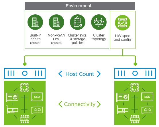
Figure 3. Discrete components in each host, and host connectivity impacts performance
Reviewing the state of the environment helps reduce the likelihood of performance issues induced by improper configuration settings or environmental conditions. It also helps identify hardware that may not be sufficient to meet the performance needs of the customer workloads. Prior to looking at specific workload and performance characteristics, a quick review of the existing topology should be performed.
Built-in vSAN Health Checks
The relevant questions would include:
- Current state of health checks: Are there any alerts?
- Initial state of health checks: Are there any alerts?
Thanks to vSAN's built-in health check framework, much of the effort to ensure proper configuration of an environment is taken care, and presented nicely within the UI, as shown in Figure 4. This performs dozens of health checks, with guidance for resolution for both vSAN specific items, as well as general vSphere related items.

Figure 4. The vSAN Health check feature in vCenter
Non-vSAN Environment Health Checks
The relevant information to discover and verify would include:
- Infrastructure Design / Switch topology
- Redundant (multiple switches) and interconnected?
- Switch make and model
- Fully copy of switch running-config available for review?
- Switches using shared buffer space for packets? (Can cause poor performance)
- Do switches have any QoS/Flow Control forced at the switch level? (invisible to vSphere, but can cause poor performance)
- Is topology using fabric extenders? (Can cause poor performance)
- Disk group verification
- Ensure correct devices are assigned for caching/buffering
- Ensure correct devices are assigned to disk group for capacity
- If using multiple HBAs on host, ensure devices in disk group use a single HBA
- Host NIC verification
- Ensure NICs are on vSAN VCG
- Ensure NICs are using latest recommended firmware
- Ensure NIC are using latest recommended driver
- Is Network Partitioning (NPAR) used?
- vSwitch configuration
- Unique IP address range for vSAN IPs
- vSAN traffic separation on switches via VLAN
- Using virtual distributed switches?
- NIOC used? What are current settings for shares?
- Sensible design based on environment?
Non-vSAN environmental checks are geared toward reviewing items are may have an impact on vSAN performance if not ideally configured. Some settings, such as network switch flow control settings may not be readily visible to a virtualization administrator, but could have a massive impact on performance. This is one reason why having complete visibility to the switchgear configuration (e.g. full copy of the running-config, topology layout, etc.) can be vital to the discovery process.
The performance of the applications can be determined by the limitations of not only the discrete hardware, but how they interact with each other, as shown in Figure 5.

Figure 5. Elements that influence performance across a topology
Cluster Data Services and VM Storage Policies
vSAN provides data services in two ways: Cluster level settings, and per-VM (or VMDK) level settings using storage policies. Both types of data services can impact the effective performance that can be delivered to a vSAN powered VM, and thus, will be important to make note of the following configuration information:
- Cluster-wide data services used
- Deduplication & Compression (space efficiency)
- Compression-only (space efficiency)
- vSAN data-at-rest encryption
- vSAN data-in-transit encryption
- vSAN iSCSI services?
- vSAN File Services
- Storage Policy rules used
- FTT1 using RAID-1 mirroring
- FTT2 using RAID-1 mirroring
- FTT3 using RAID-1 mirroring
- FTT1 using RAID-5 erasure coding (space efficiency)
- FTT2 using RAID-6 erasure coding (space efficiency)
- IOPS limit for object (can cause higher latencies when enforced)
- Number of disk stripes per object
- Secondary levels of protection, such as in stretched clusters, and in 2-node clusters (introduced in vSAN 7 U3)
Cluster-wide data services may affect the amount of processing for the I/Os in the data path for the entire cluster. This is most applicable to data services such as Deduplication and Compression, vSAN data-at-rest encryption, and vSAN data-in-transit encryption. They data services listed above are linked to blog posts that detail the performance implications of each service. See the post: Performance when using vSAN Encryption Services for more information.
Storage policy rules applied at a per VM or per VMDK level in order to provide various levels of failure to tolerate impart different levels of effort to process data. An example of this Is the effect a storage policy has on I/O amplification. In Figure 6, we see the differences in I/O amplification when choosing various levels of data protection and space-efficiency assigned using a storage policy.

Figure 6. I/O amplification for write operations, when choosing levels of data protection and space-efficiency
I/O amplification Is a term used to describe a storage system issuing a multiplier of I/O commands for every I/O command issued by the guest physical or virtual machine. The amplification is the result of the storage system providing a defined level of resilience, performance, or some other data service. Many storage systems do not provide any visibility to the underlying I/O amplification. vSAN provides a significant amount of detail around this, courtesy of the graphs In the vSAN Performance Service.
I/O amplification exists with any storage architecture, but with HCI, write operations are sent synchronously to more than one host. This means that the write latency is only as low as the slowest path to the remote host. This amplification can also occur even more in conditions where one is using a secondary level of resilience, such as a stretched cluster or 2-node clusters. See the posts: Performance with vSAN Stretched Clusters and Sizing Considerations with 2-Node vSAN Clusters running vSAN 7 U3 for more information.
Cluster Topology
vSAN allows for administrators to accommodate for their business objectives in combination with the physical topology of the data center. This can show up in several ways.
- vSAN stretched clusters. The use of a single vSAN cluster stretched across physical sites ensures that data remains available in the event that one of the physical sites is unavailable.
- vSAN explicit fault domains. The use of explicitly defined fault domains (e.g. Rack or room), ensures that data remains available in the event of a single host, or a group of hosts such as a rack or data closet is unavailable.
- HCI Mesh. This allows for storage capacity from a single vSAN cluster to be used VMs in other vSAN clusters, or traditional vSphere clusters. This provides more flexibility for resource utilization and consumption of data services.
For more information, see the post: How vSAN Cluster Topologies Change Network Traffic. When reviewing the topology, consider how any of the capabilities described above can potentially impact performance. For example:
- A vSAN stretched cluster can impact performance as a result of needing to commit synchronous writes across an inter site link (ISL). This ISL is often the most constraining part of the storage stack. This assumes that the respective storage policy for a VM is using the “dual site mirroring” rule to provide site-level redundancy. See the post: Performance with vSAN Stretched Clusters for more information.
- Clusters using explicit fault domains, or HCI Mesh can change the path that data uses to traverse to the respective host(s). These clusters are more likely to span traffic across top-of-rack (ToR) leaf switches, and onto the spine. Therefore, sufficient network latency minimums and bandwidth at the leaf AND spine levels must be available to ensure minimal impact on performance. vSAN traffic extending beyond the ToR leaf switches and onto the spine can also occur with larger vSAN clusters. ToR switches can typically only support a certain number of hosts, which means that traffic will arbitrarily traverse across the spine to connect to the other racks.
- HCI Mesh can complicate the performance troubleshooting process because the contributing factors could come from the HCI Mesh server cluster, the HCI Mesh Client cluster, or the switching fabric (beyond ToR leaf switches) that connect the clusters together. Proper isolation strategies can help simplify this troubleshooting process.
Note that environments running stretched clusters using previous editions of vSAN would refer to the protection setting across a site as a “Primary Level of Failures to Tolerate,” or PFTT. All recent versions of vSAN use the term "site disaster tolerance" as reflected in the user interface.
Hardware Specs and Configuration
The relevant hardware information to discover and verify would include:
- Cluster Characteristics
- vSAN ReadyNodes, VxRail, or build-your-own?
- Number of hosts in cluster
- CPU/Mem (per host)
- Disk group layout
- Number of disk groups per host
- Number of capacity devices per disk group)
- Buffering tier hardware (SAS? NVMe)
- Capacity tier hardware (SATA, SAS, NVMe?)
- Disk Controller used (# per host, and make/model)
- Using any SAS expanders?
- NIC type, speed, and number of uplinks?
- Uplinks using LAGs?
- Current amount of free space in cluster?
- Was performance a primary requirement on the initial BoM, or was it price?
- Has It been verified that all hardware Is on the VMware Hardware Compatibility Guide (VCG) for vSAN? If so, what hardware has been Identified as not being on the compatibility guide?
- Are hosts that comprise a cluster providing a relatively balanced set of resources? (CPU, RAM, host NICs, storage capacity, number of disk groups, etc.)
Basic hardware checks might sound unnecessary, but double checking hardware is often the time in which a user discovers that perhaps the hardware being used was not what was intended, or are seeing the reality of the initial bill of materials specification. For example, a cluster may consist of hosts that use cost effective, but lower performing SATA based SSDs for a capacity tier as opposed to higher performing SAS. Or perhaps an NVMe device wasn't properly claimed as the buffering device.
The image shown in Figure 7 represents the cost/performance/capacity pyramid of storage device types. The device types choses will contribute to determining the speeds that vSAN will be capable of. Similar price and performance tradeoffs exist for network connectivity, CPU, and memory.

Figure 7. The cost/performance/capacity pyramid of storage device types for vSAN
The number of hosts in a cluster can play an important role in vSAN's ability to provide desired level of resilience, and performance. For more information on understanding the tradeoffs between environments using few vSAN clusters with a larger number of hosts, versus a larger number of vSAN clusters with a few number of hosts, see: vSAN Cluster Design - Large Clusters Versus Small Clusters and the blog post: Performance Capabilities in Relation to Cluster Size.
Step #3: Discovery/Review - Workload
Get a better understanding of the applications, processes, and workflows that are running on the vSAN powered environment.
Once the environmental checks are out of the way, discovery efforts can focus on the applications and workloads at play. We break this discovery down into two categories: application characteristics, and workflow/process characteristics. These categories are necessary for review because, as newer hardware is introduced into an environment, one may find that some performance bottlenecks may exist with the applications, and what are demanded of them: The processes and workflows that are used by an organization.
The "application characteristics" category simply represents the applications at play, the quantity, guest VM configuration settings, storage policy settings, and anything else that may impact performance. The "workflow/process characteristics" category aims to discover what activity is being demanded of the application. It is the combination of the two that made the demand on your environment unique. Remember that the demand on resources by an application primarily depends on what is being asked of it. An environment could have dozens of SQL server VMs, but if there is nothing being asked of them, they will create very little load on an environment.
Applications
The relevant VM and application characteristics information to discover would include:
- What is the application(s) that are not sufficiently meeting performance expectations?
- Does app run as single instance, or part of farm (e.g. single SQL VM vs cluster)
- Does app depend on other VMs?
- Are other VMs dependent upon this app (e.g. part of multi-tier solution)
- What type of VM or in-guest configuration settings were done for deployment the specified application/OS.
- Multiple VMDKs?
- Multiple virtual SCSI controllers to distribute VMDKs amongst.
- Memory reservations
- Number of vCPUs
- vSAN settings associated with this VM (also mentioned in "Cluster Data Services, and VM Storage Policies" in step #2)
- What type of storage policy is being used by VM?
- What type of data services are being used on the cluster powering the VM (e.g. DD&C, encryption, etc.)
- Are there other applications or workloads that might impede performance of these business critical applications?
- Data protection methods such as backups
- Frequent and/or large reindexing activities
- Data transformation services
Applications often have a number limits that prevent performance to increase at the same rate that the underlying hardware offers. For example, many multithreaded applications become single threaded during storage I/O activities. It is also not uncommon to see that recommended deployment practices of a given OS and application were not followed, which prevents optimal performance of an application. Commonly overlooked optimizations include the use of multiple VMDKs with their own virtual paravirtual SCSI controller in order to take advantage of I/O queuing across multiple virtual disk controllers, as opposed to a single virtual controller. For a list of other common VM tuning options, see the "Applications" portion of the Step 5: Mitigation.
Workflow and Processes
The relevant workflow and process characteristics information to discover would include:
- What type of tasks, or workflow is being performed on application?
- Batch process at fixed intervals? If so, how often, and how long to completion?
- Have workflow tasks been mapped to better understand business objectives? (often needed because old, potentially inefficient workflows live on in perpetuity)
- e.g. department y needs database replicated 3 times per day, and SSIS is run to perform a bulk update at desired frequency.
- Does given workflow have a dependency of multiple VMs in order to achieve desired result?
- How is the VM being measured to determine whether or not it is able to meet expectations?
- Guest VM latency?
- Time to complete given workflow
- Is given workload highly transactional (serialized)? SQL are good examples of this, and can be highly influenced on latency.
Overlooking automated workflows and processes inside an organization can often undermine an otherwise well designed infrastructure. The workflows in place were often originally built for processing an moving much smaller amounts of data than what may currently exist in the environment. Some processes can become extremely inefficient at scale. Figure 8 uses the example of database replication that was occurring inside the application, and using a bulk, full copy process inside of the main datacenter, and across multiple sites. Moving to a transactional update type of a workflow would result in much less data movement and resource usage, thus no longer being constrained in time by the method used. Moving to vSAN and reviewing processes complement each other, as the aggregate performance improvement can be substantial.

Figure 8. Legacy workflows can carry a heavy resource burden, and can be tuned using newer techniques and tools.
You may find that the application owners and/or administrators may provide valuable insight as to what is being asked of the application. They may be aware of automated processes, stored procedures, or some other event driven tasks that can help explain behavior of an application. Closely monitoring performance activity of applications in a data center can often provide a great point of reference for unusually large resource usage.
Step #4: Performance Metrics – Insight
Taking the first steps to measure performance characteristics of a workload, and the environment it lives in.
As noted earlier, while a traditional top-down approach can be used for the identification of a performance bottleneck, the nature of vSANs distributed storage introduces additional considerations when attempting to diagnose performance issues.
Performance metrics will be the most helpful way to quantify the performance of current and past conditions, and to visualize the capabilities of your environment. Most importantly, time-based performance metrics provide an understanding of behavior during a period of time. For example, measuring the time to completion of a SQL batch process may be the most important measurement to the business, but it does not provide the context that allows the user to see change in performance behavior may be occurring, and if those performance impediments are occurring because of the underlying hardware, or other processes.
Understanding time-based measurements
Monitoring systems typically collect a series of data over a period of time, sometimes known as a "sampling rate" or "collection interval." Through the use of counters, it is able to determine how much activity occurred over that period of time, and presents that as a single value that represents an average. For instance, if a tool measuring I/O operations per second (IOPS) had a 1 minute sampling rate, it will count the sum total of I/Os over the course of the 1 minute sampling rate, then divide that by the total number of seconds (60) in that period. If it was measuring latency, it would take the total delay over the sampling interval, then divide that by the total number of I/Os in that period. This practice is in place to reduce the potentially massive amount of resources used simply for data collection and retention.
vCenter performance statistics (those that show up whether the infrastructure uses a traditional three tier storage, or vSAN) use a graduated sampling rate. For the first hour, most metrics will use a sampling rate of 20 seconds. Once the data is older than 1 hour, it will be rolled up, or resampled to 5 minute intervals. When the data is older than one day, the performance statistics will be rolled up to 30 minute sampling intervals, and stored for 1 week. Beyond one week, samples will be rolled up to 2 hours and stored for 1 month. All samples beyond 30 days will be rolled up to 1 day and stored for one year. This means that the data may be less meaningful over the course of time because it loses the level of granularity needed to see variations in performance.
VMware Aria Operations gathers performance metrics using vCenter APIs. By default it will use a 5 minute sampling rate, and will retain performance data for a default duration of 6 months. In comparison to vCenter, it makes the compromise of longer sampling rates for recent time windows (e.g. 1 hour) for the benefit of fewer data rollup actions over the life of the data retention period. This approach better suites its trending/analysis capabilities. Sampling rates in VMware Aria Operations can be reduced to 1 minute, but this is not recommended due to the load it can generate. For more information on VMware Aria Operations in vSAN environments, see the VMware Aria Operations Suite in vSAN Environments guide. When transitioning workloads to vSAN, either the native vCenter performance statistics, or VMware Aria Operations can be used for comparison of key performance metrics after the migration. VMware Aria Operations has a "Migrate to vSAN" (known as "Optimize vSAN Deployments" in older versions) dashboard that provides the ability to compare two similar VMs, one on vSAN, and one on traditional storage.
Unlike typical ESXi host and VM metrics collected by vCenter, the vSAN performance service is responsible for collecting vSAN performance metrics in a cluster. It is stored as an object, and distributed across the cluster in accordance to the storage policy assigned to it. The vSAN performance service can render a time window from 1 hour to 24 hours using a 5 minute sampling rate, and can retain performance data for up to 90 days. While this data is presented in vCenter (always under the Monitor > vSAN > Performance area for the VM, host, or cluster), it remains independent from vCenter, and does not place any additional burden on vCenter resources. It presents VM performance metrics only for those running on a vSAN datastore.
Comparing the same performance data using dissimilar sample rates can produce inconsistent results. In the image shown in Figure 9, we see measuring the very same data with different sampling rates can present different results. Not only do the sampling rates affect the top-line number, but they also change in shape, due to the finer level of granularity with a smaller sampling rate. They are all accurate for how the measurement is defined, but should not be used to compare to each other. Longer sampling rates may miss a spike simply because the duration was less than the time period used for the collection interval, which would dramatically reduce the calculated average.

Figure 9. How sampling rate can change perceived result of performance metrics
Sample rates can also Impact the perception of activity for VMs with lower levels of I/O. For example, a VM might display 0 read IOPS when viewing In a performance graph using a 5 minute sampling Interval. The VM may have had several read I/Os during that sampling period, but not enough to meet an average of greater than zero over that 5 minute sampling period. This "trickle I/O" can occasionally cause phantom latency, as described later in this document in "What to look for" section near Figure 11.
Changing the time windows (the period of interest) for given metrics is also a valuable technique. For more information, see the post: Changing Time Windows for Better Insight with Performance Metrics for vSAN and vSphere
What you measure, how you measure, and where you measure it can dramatically influence the result and supporting conclusions. Understanding this step can help identify and quantify performance challenges. Let's look at this in more detail.
What to measure
There is no shortage of performance indicators to measure. For the purpose of better understanding storage I/O activity and performance, three metrics will be the ideal starting point.
IOPS
This measures the number if storage I/O commands completed per second. I/Os from the guest VMs are only a result of what the guest VM, and it's applications are requesting. The less latency there is throughout the storage stack, the more potential there is for a higher rate of IOPS.
IOPS measured by the hypervisor may be different than measurements inside the guest, or if using traditional storage, at a storage array. Guest operating systems can coalesce writes into one larger write I/O prior to be sent to the storage subsystem, and storage arrays may have their own methods to process the data which can impact the rate reported. This is why it is best to standardize the location of measurement to be the hypervisor.
Throughput
Throughput is the volume of storage payload transmitted or processed. It is typically reported in KiloBytes per second (KBps). Throughput is the result of IOPS multiplied by the respective sizes of the individual I/Os. Changes in throughput can be a reflection of a change of IOPS, or the relative sizes of the I/Os being processed. I/O sizes can vary dramatically, and due to this, can influence performance significantly. More on this later in this document.
Latency
Storage latency is the time to complete/acknowledge the I/O delivery, and is typically reported in time in milliseconds (ms). It is the time the system has to wait to process subsequent I/Os, or execute other commands waiting for that I/O. With the hypervisor, latency measurements can be taken for just a portion of the storage stack (visible via ESXTOP), or the entire end-to-end path: from the VM, to the storage device. Note that latency is a conditional metric. It gives no context to the amount of I/Os that are feeling that latency. A VM that averages 10 IOPS with 20ms of latency may not be as concerning as a VM demanding 700 IOPS with 15ms of latency. Unlike IOPS or throughput, where total VM IOPS or throughput is a sum of the read and write IOPS, using the same method for VM total latency may produce misleading results. Therefore, it is best to view latency always as two distinct measurements: Read latency and write latency.
Just as with IOPS and throughput, it is typically best to measure latency of the guest VM and/or VMDK at the hypervisor level. There can be times that monitoring latency inside the guest using the OS monitoring tools can be useful. The disparity between the VM or VMDK latency and disk latency inside the guest can sometimes be the result of exhausted queue depths of non-paravirtual controllers that use lower queue depths. More on this topic later in the document.
What to look for
The workloads will dictate the I/O demand (IOPS or throughput), and will likely be bursty in nature. This is normal, and controlled entirely by the application and its processes. The periods in which I/O bursts may be artificially suppressed is when there are substantial amounts of latency during the same time period. With a few exceptions (e.g. heavily used VMs with continuous jobs to perform), a VM running a real production workload with optimally performing storage will not always show a higher average of IOPS than the same environment with lesser performing storage. Contrast this with synthetic I/O testing, where faster storage typically equates to higher IOPS. For real workloads, the optimally performing environment simply allows the tasks and workflows to be completed more quickly. Tasks completed more quickly will be offset by periods of lower activity, sometimes within the collection interval of the metric, and is the reason why average IOPS reported may not necessarily increase on a newer storage system demonstrating lower latency.
When looking for opportunities in performance improvement with real workloads in a vSAN environment, latency will be the most important measurement to base conclusions. When evaluating latency, two elements that the reader should look for is low latency, and consistency of the latency. High latency periods are opportunities for improvement. It is an indicator that the VMs, and the applications that run in them are waiting on the storage to continue its operations.
What is high latency, and what is low latency? High and low latency really are dependent on the inherent capabilities of the collection of discrete hardware devices (storage devices, controllers, network cards), the hypervisor, the guest operating system, and the in-guest applications. A vSAN cluster that powered by entry-level SATA flash devices, low-end networking, and an older version of vSAN will not be nearly as capable as a vSAN cluster that using NVMe devices, 25Gb networking, and the latest version of vSAN. Storage latency will result in applications completing tasks more slowly. Some applications may be more sensitive to latency than others, and may result in timeout requests or introduce errors.
When monitoring real applications in production environments, latency is the symptom that tells you there is opportunity to improve overall performance by storage optimizations. If storage latency is low and consistent, it can be deemed as not the current bottleneck. The bottlenecks may exist inside the application, the workflows, CPU, or elsewhere. Note that latencies with real workloads may be higher than demonstrated with synthetic testing. This is typically due to real workloads using much larger I/O sizes than used in synthetic testing. See Appendix A for more information.

Figure 10. Observing write IOPS and write latency of a VMDK in vCenter
Measuring I/O latency requires I/O activity to measure against. If it does not exist, then measurements can occasionally be misleading. In Figure 11, we see that read latency is showing a noticeably higher number on the first period of the graph. Notice the corresponding IOPS in this 4-node cluster was just 1 read I/O per second. In a 4-node cluster, this means that there were not enough read I/Os across that sampling period to measure the latency against, thus generating a misleading number. This low number of I/O, sometimes referred to as "trickle I/O" can occasionally generate false latency spikes on any type of shared storage. This phenomenon of phantom latency may be seen at the cluster level, or down to even the individual VMDK. This is a great example of why a single metric such as latency should not be looked at in isolation. Correlating latency back to the amount of activity occuring is a good way to provide context, and elliminate false positives.

Figure 11. Phantom latency may occur when there is little to no I/O activity.
Relationship of Metrics
These metrics have an indelible tie to one another, and should be looked at together when viewing the behavior of VMs in an environment. IOPS indicates the level of activity, but not the size of the payload. Throughput indicates the size of the payload, but not the level of activity. Latency dictates the limit of IOPS and throughput that the VM is able to process in the environment it is powered by.
The emphasis of IOPS, throughput, and latency should not diminish the importance of other metrics. The plethora of other metrics available are in large part to offer more insight at various levels in the stack, with some described in Appendix A of this document. They should be viewed as supporting data to the primary measurements indicated above. Note that IOPS, throughput, and latency can be measured at the VM, at the host, at the cluster level, along with a number of other conditions. This will be covered in the "Where to measure" in the next section.
Where to measure
Historically, users have had numerous options on where to measure performance data. Inside, the guest, at various layers of the hypervisor, and when using traditional three-tier storage, at the storage array. This flexibility causes a substantial amount of confusion, as measuring from the wrong, or inconsistent locations can produce incomplete, or inaccurate results. For example, storage arrays do not have end-to-end insight to the entire storage path the VM uses. Measuring data inside the VM can sometimes be equally as challenging. Operating systems' method of data collection assumes sole proprietorship of resource, and may not always accurately account for the sharing of resources. Using multiple locations for measurement also assumes that the definitions for the metrics such as IOPS, throughput, and latency are exactly the same. Often they are not.
Therefore, the user needs a common monitoring plane for interpretation of performance metrics. vCenter has always offered the ideal monitoring plane, as it normalizes the definitions of all metrics, and is pulled from the most intelligent location in the stack: The hypervisor. Even more so with vSAN, as it provides a storage system that is integrated into the hypervisor. For the end user, this means that with vSAN powered environments, vCenter can see and control storage from end-to-end. Using vCenter also provides another benefit: Acting as a common substrate for further analysis. APIs are used by infrastructure analytics solutions like VMware Aria Operations to fetch the same data seen in vCenter. This is critical to ensuring that data using the same definition and source are used.
Now that we've established the ideal location for measurement (they hypervisor), let's look at the most critical levels of measurement for understanding workloads, and the cluster powering them.
Guest VM level (and Virtual Disk)
Application and OS behaviors tied to the VM can be viewed at the guest VM level. Metrics such as IOPS, throughput and latency can be viewed at this level, and will establish an understanding of the effective behavior that your critical VM is seeing at the ESXi vSCSI layer, isolating the source more quickly. These metrics can be viewed in two ways. One can highlight the VM, click on Monitor > Performance > Advanced > Virtual Disk, then customize the chart as needed. It will also render performance metrics at a high 20 second sampling rate for the first hour. Another method of measurement can be done by highlighting the VM, clicking on Monitor > vSAN > Performance, and then selecting the aggregate VM tab, or the Virtual Disks tab for analysis of independent virtual disks for the VM. This data comes from the vSAN performance service.

Figure 12. vSAN performance service metrics at the VM level
Cluster level
Measuring at the cluster level provides context, and helps identify influencing factors. Remember that vSAN is a cluster based storage solution, and VM data is not necessarily always residing on the host that the VM is residing. While it might seem odd to check look at performance metrics at this level as the second step, it can often help provide an understanding to the level of activity across the cluster. For example, perhaps a VM latency spikes occur during the middle of the night. After identifying the VM level statistics, viewing the cluster level statistics might show a substantial amount of noise coming from other VMs, or perhaps backend resynchronization traffic. To view the vSAN cluster based performance metrics, highlight the cluster, click on Monitor > vSAN > Performance to view the respective VM, backend, or iSCSI performance metrics.

Figure 13. vSAN performance service metrics at the vSAN cluster level
In vSAN 7 U3, the VM I/O trip analyzer can play a useful role in determining where the potential bottleneck may exist in the storage stack. By selecting a given VMDK and determining the period of time of monitoring, it will render a visual map of the I/O stack and indicate where it determines contention may be occuring, such as the capacity device, the buffer device, the NIC, etc.
Host level
This is the next level to for viewing, and will offer up the most levels of detail. Host level statistics should be viewed once it has been established on where the objects for the individual VMs are located at in the cluster. To determine this, highlight the VM in question, click on Monitor > vSAN > Physical Disk Placement. Once the appropriate host has been highlighted, click Monitor > vSAN > Performance. This will expose the following:
- VM level statistics (aggregate of all VM objects on the host.)
- Backend vSAN statistics
- Physical disks and disk groups (discussed in more detail in step 4)
- Physical Network adapters
- Host Network and vSAN VMkernel activity
- iSCSI service activity

Figure 14. vSAN performance service metrics at the host level.
Storage devices and disk groups
Through host level statistics, vSAN exposes key information about disk groups. Since a disk group is comprised of at least one caching/buffering device, and one or more capacity devices, this view can expose a lot of insight into the behavior of an environment, including, but not limited to cache disk destage rates, write buffer free percentages, and the different types of congestions. Performance data can be viewed from the disk group in its entirety, from the caching/buffering device servicing a disk group, or from a capacity device serving a disk group.

Figure 15. Performance metrics of a disk group on a vSAN host.
See KB 2144493 for a complete listing of vSAN performance graphs in vCenter. Key metrics will be discussed in detail later in this document. For more information on the different levels of vSAN performance metrics, see the post: Performance Troubleshooting - Understanding the Different Levels of vSAN Performance Metrics
For a better understanding of which metrics should be viewed first, see the post: Performance Troubleshooting - Which vSAN Performance Metrics Should be Looked at First?
How to measure
Ideally, one would want to collect time based activity in the form of graphs, representing the time windows most relevant for the diagnosis. In light of the known sampling rates in vCenter, in the vSAN performance Service, and in VMware Aria Operations, a good starting point may be to collect the following based on the circumstances:
- Previous 1 hour
- Previous 8 hours
- Previous 24 hours
- Known duty cycle of a process or workflow within an application
Capturing these time periods can help provide and understanding the demands placed on the VM. Since time-based graphs provide great context to the behavior of the demand, a simple, but highly effective approach when diagnosing performance issues are to capture the metrics using screen shots. For example, screenshots could be taken of a VM's "real-time" metrics that only have a 1 hour lifespan in vCenter, and used to compare it to real-time statistics at a later time. This is also effective for looking for correlations between performance changes that occur at a disk group level, a host level, or a cluster level. Captured images of time-based graphs can also be used for "before and after" comparisons once mitigation efforts are underway.
When viewing vSAN based metrics in the performance service, one can save a given time range. This feature can be helpful when navigating through various performance metrics.
Finding the VMs/Apps in question
Determining the applications that are experiencing storage performance issues can come from multiple sources. Sometimes it will be batch process notifications coming in later than usual, or user complaints. vCenter can be used to discover storage latency issues, but is not optimal for quickly determining which VMs are experience the most latency. VMware Aria Operations does an excellent job of collecting and enumerating guest VMs by the highest average latency, or any other metric desired. PowerCLI scripts can also be used to achieve a similar result.
Caution needs to be exercised when identifying VMs by average latency over the course of a given time window.
- Latency with discrete workloads typically shows up as spikes. Capturing average VM latency on over a window of time may not be representative of the behavior, due the calculated average being heavily influenced by the other sample periods.
- Measuring read or write latency of a VM, with multiple VMDKs may obfuscate the issue, due to the calculated average being heavily influenced from the other VMDKs associated with the VM.
- Application characteristics, and demands of the workload may naturally induce higher latencies. For instance, a file server may be writing data using large I/O sizes, which will have a significant higher latency than another workload, using smaller I/O sizes.
Some tools allow for measuring latency peaks. This unfortunately isn't ideal, as it can unfairly represent statistical outliers, which may very well occur when there is little to no I/O activity. The best way to understand the actual behavior of VM and application latencies is to observe in time based performance graphs. Depending on the level of detail, you may need to measure at the individual VMDK level. Become familiar with these graphs to determine what is normal, and what is not for that given application. This is where you can use built-in functionality of vCenter and the vSAN performance service metrics to gather this information
vSAN 7 U1 and vSAN 7 U2 introduce new ways of quickly viewing the most demanding VMs in a cluster, and comparing them against other systems. Figure 16 shows the top contributors for a specific point in time to quickly determine the VMs demanding the most resources. For more information, see the posts: VM Consolidated Performance View in vSAN 7 U1 and Performance Monitoring Enhancements in vSAN 7 U2.

Figure 16. The "Top Contributors" cluster view in vCenter Server.
Being familiar with typical latencies by a VM using time-based graphs will help clarify performance characteristics that are normal and abnormal for the environment.
Step #5: Mitigation - Options in potential software and hardware changes
Actionable steps to help address performance issues based on the symptoms, and addressing the most significant source.
With the data gathered using the methods describe in the earlier steps, one has all the information necessary to take action on some of the performance issues that may be seen in an environment. The information below describes an assortment of options that will help improve the performance of one or more VMs running in a vSAN environment. They are categorized in the same "discovery" categories shown in Figure 2 at the beginning of this document.
The options provided In each category are presented In no particular order, as the available options may be dependent on business requirements, and the degree of improvement that one is seeking. For example, in some situations, a user may be able to achieve the desired performance requirements through a software change, such as adjusting a storage policy on a VM. In other situations, a user may only be able to achieve the desired requirements through the purchase of higher performing hardware.
While high guest VM latency is the leading indicator for opportunities for performance improvement, the causes can be for many reasons. Without delving deep into a variety of subsystems, there is no simple correlation that will always pinpoint the exact bottleneck, or the amount of degradation that it is introducing. The categories below should help address performance issue identified.
Mitigating Network Connectivity Issues in a vSAN cluster
Some of the mitigation options listed below relate to the components or configuration of the network used by vSAN. As with any type of distributed storage system, VMware vSAN is highly dependent on the network to provide reliable and consistent communication between hosts in a cluster. When network communication is degraded, impacts may not only be seen in the expected performance of the VMs in the cluster but also with vSAN's automated mechanisms that ensure data remains available and resilient in a timely manner.
In this type of topology, issues unrelated to vSAN can lead to the potential of a systemic issue across the cluster because of vSAN's dependence on the network. Examples include improper firmware or drivers for the network cards used on the hosts throughout the cluster, or perhaps configuration changes in the switchgear that are not ideal. Leading indicators of such issues include:
- Much higher storage latency than previously experienced. This would generally be viewed at the cluster level, by highlighting the cluster, clicking Monitor > vSAN > Performance and observing the latency.
- Noticeably high levels of network packet loss. Degradations in storage performance may be related to increased levels of packet loss occurring on the network used by vSAN. Recent editions of vSAN have enhanced levels of network monitoring and can be viewed by highlighting a host, clicking on vSAN > Performance > Physical Adapters, and looking at the relevant packet loss and drop rates.
Remediation of such issues may require care to minimize potential disruption and expedite the correction. When the above conditions are observed, VMware recommends holding off on any corrective actions such as host restarts and reaching out to VMware Global Support Services (GS) for further assistance.
Built-in vSAN Health Checks
Upgrade vSAN to the latest version
VMware makes continual improvements in the performance and robustness of vSAN. For example, in vSAN 7 U1 introduced several performance optimizations, including a new performance focused "Compression-only" space efficiency feature. vSAN 7 U2 introduces the support of RDMA, and new optimizations for VMs using RAID-5/6 erasure coding. Simply upgrading to the newest version of vSAN may dramatically increase the performance of the workloads running in a vSAN cluster. Remember that upgrades can occur on a per-cluster basis, so they can be tested and phased in gradually.
Resolve any outstanding environment/configuration items discovered in step 2
Many of the health checks exist to alert the users to configuration or environmental findings that may impact performance or stability in the environment. When highlighting an health check alert, be sure to click on the "Ask VMware" link in the "information" section of the specific health check. This will connect to a KB article giving more information, and sometimes prescriptive guidance on the issue described.
Assess options for clusters nearing capacity full conditions
vSAN clusters going beyond the recommended capacity utilization settings can generate cause more backend I/O activity than clusters under this threshold. Minimizing backend I/O activity can potentially improve the consistency of performance that vSAN can deliver. Capacity can be increased by adding hosts, or adding storage devices. Note that free space recommendations have changed in recent editions of vSAN. For more information, see this section of the vSAN Operations Guide.
Non-vSAN Environment Health Checks
Ensure the appropriate firmware and drivers are used for host NICs
A number of performance and connectivity issues have been traced back to NIC firmware and associated drivers. Very capable hardware can show quite poorly simply due to bad NIC firmware, and/or drivers. While some NIC driver health checks have begun to show up in the built-in health checks, this is very limited. It is highly recommended to ensure the host NICs are running the latest approved firmware, and associated drivers.
Switchgear class
VMware does not provide any qualified list of approved switches for vSAN or any other solution. vSAN heavily depends on network communication to present distributed storage to the cluster, and therefore, the class of switches chosen can be critically important to the performance capabilities of vSAN. Switchgear have different performance capabilities that go far beyond the advertised port speed. For switchgear supporting a vSAN environment, look for enterprise grade, storage-class switchgear using large dedicated port buffers, as well as sufficient processing and backplane bandwidth to ensure that each connection can run at the advertised wire-speed.
The use of fabric extenders can result in a non-optimal communication path, and are not recommended for storage fabrics, including vSAN.
Switchgear settings
Switch setting can have port based or global settings that may be invisible to the virtualization administrator, but can impact the performance of an environment. For example, QoS/flow control managed on the switch can throttle effective throughput for devices connect to the ports, yet the ports will still advertise the full link speed. For these reasons, it is recommended to rely on flow control mechanisms in the hypervisor instead.
Other switchgear settings may be a byproduct of the physical capabilities of a switch, and impart significant performance penalties on the environment. For example, one enterprise grade switch uses a shared buffer space across ports. This port buffer space is then controlled through switch settings. The default setting of the switch limits port buffer to a very small size of 500KB. It provides an option to increase this to 2MB, or to allow for the highest possible size for the shared buffer. The latter is the most desired setting. Switches that use this type of artificial limit for shared port buffers would act similar to small port buffers found in non-enterprise grade switches. Both would result in significant amount of dropped packets, and retransmits. This wastes CPU cycles on the host, and will show up as potentially high levels of guest VM storage latency.
Ensure use and settings of NIOC for vSAN using non-dedicated uplinks
Using Network I/O Control (NIOC) will ensure a fair distribution of a shared network resource under periods of contention. The vSAN Design and Sizing Guide mentions this feature, and vSAN Network Design Guide demonstrates enabling NIOC, as well as providing a configuration example.
Ensure Network Partitioning (NPAR) Is not used on links serving vSAN traffic
NPAR is a network partitioning feature of host NICs that can present a single physical NIC port as multiple ports. It can restrict the maximum bandwidth available to these ports even during periods of no contention. The effects of NPAR can undermine an otherwise capable cluster, while being relatively undetectable to the virtualization administrator. If traffic shaping is needed to provide shared bandwidth for non-dedicated links, use NIOC instead.
Jumbo Frames
As described in this section of the vSAN Network Design Guide, vSAN supports MTU sizes beyond 1500 bytes. Using jumbo frames can reduce the number of packets transmitted per I/O. This effectively reduces CPU overhead needed for transmitting network traffic, and may improve throughput. It may not have any impact on storage latency as seen by the VM. For environments that do not use larger MTU sizes, implementation may introduce significant levels of effort to ensure the larger MTU sizes are operating correctly end to end. Since increasing MTU sizes may have a less significant impact than other changes, it may be best to consider other opportunities for improvement prior to implementing jumbo frames.
Check BIOS power savings settings
Set the Host Power Management to 'OS Controlled' in the Server BIOS for the duration of the performance test. Verify that the setting has taken effect by checking the Power Management of the host in the vSphere client. Technology should show APCI P-States and C-states, and the active policy should show 'High performance'. See the "Performance Best Practices for vSphere" for the latest guidance on host power management settings, and KB 1030265 for guidance on interrupt mapping.
Cluster Data Services and VM Storage Policies
Adjust storage policy settings on targeted VM(s) to accommodate performance requirements
A quick an easy adjustment for VMs not meeting performance expectations is to assign a new storage policy using a data placement and protection scheme that generates less I/O amplification than the currently selected policy. This can be performed without any downtime, and once the resynchronizations are complete and the VM(s) are using the new storage policy, one can observe the effective results in the performance graphs to see if it meets latency expectations. An explanation of I/O amplification can be found in section “Step #2 – Discovery/Review - Environment” of this document, along with an illustration found in Figure 6 comparing I/O amplification as it relates to storage policies. Remember that storage policies can be applied on a per VM, or even per VMDK basis. For example, a SQL server VM using a storage policy of RAID-6 erasure coding could have just the database and transaction log VMDKs changed to a storage policy using RAID-1 mirroring. Depending on where the effective bottleneck lives in a given infrastructure, changing a VM's storage policy from using RAID-5/6 erasure coding to RAID-1 mirroring can have a noticeable improvement in performance when networking or other resources may be a bottleneck.
One can test to observe if there are any performance improvements by applying a storage policy using a stripe width of greater than 1 to the target VM. Leaving the stripe width to the default of 1 is generally recommended, but in certain circumstance, providing a stripe width of greater than one may help with performance. See the post: RAID-5/6 Erasure Coding Enhancements in vSAN 7 U2 for more information on recent enhancements performance enhancements with erasure coding, and Stripe Width Improvements in vSAN 7 U1 for more information on stripe width setting changes in vSAN.
Adjust storage policy settings on non-targeted VM(s) to reduce I/O amplification across cluster
This is similar to the recommendation above, but instead of making a storage policy adjustment to the application with the performance issue, one could review the storage policies used by other VMs in the cluster. For example, one may find a large majority of VMs in a cluster using a RAID-6 based storage policy. RAID-6 offers a high level of protection while simultaneously being space efficient, but can introduce much more I/O amplification and network traffic when compared with other data placement strategies. To experiment, one could create a new storage policy, take the busiest VMs (top 30%, 50%, or whatever desired), and assign these VMs to that new storage policy to reduce their burden on the environment. After the VMs have had the policies successfully applied to them, one can view the performance graphs (primarily, guest latency) to see if there was any beneficial result.
Stretched clusters environments that use storage policies that define secondary levels of resilience may impact the effective performance of a VM if the hosts and topology have not been designed for such a configuration. See the post: Performance with vSAN Stretched Clusters for more information.
Adjust cluster-wide vSAN data services to accommodate performance requirements
Cluster-wide data services can be easily turned on or off on a per cluster basis. These data services offer extensive capabilities, but may impact storage performance. A cluster with one or all of these services turned off will generally be capable of providing better performance than those that use these services. Each service has the following impact:
- Deduplication & Compression: All writes are committed to the write buffer in the same way writes are committed with this service turned off. Therefore, in cases where there is not significant pressure in destaging, the guest VM will generally not see additional write latency. The additional effort (CPU cycles, and time) to destage data will increase, equating somewhat to a slower capacity device. If the write buffer has rate of incoming writes for a prolonged period of time, and that cannot be met by a sufficient destage rate, the buffer will near its capacity, and write latencies may eventually be impacted. Reads, especially those fetched from the capacity tier may be impacted, but in a less significant, and less predictable way. The service consumes host resources (memory and CPU), and may have some impact on density of VMs per host. For customers interested in using opportunistic space efficiency, Deduplication & Compression should only be used under a limited set of conditions and use cases.
- Compression-only: All writes are committed to the write buffer in the same way as described above. With Compression-only, the compression occurs on destaging, with much less computational effort, and thus, a faster rate of destaging when compared to DD&C. For customers interested in using opportunistic space efficiency, Compression-only should be the default space efficiency feature used, as it is appropriate for most workloads with minimal computational effort.
- Data-at-rest encryption: For writes, vSAN will encrypt the data as it lands in the write buffer, and go through the process of decryption and encryption when it is destaged to the capacity tier. For reads, decryption occurs whether the data is read from the write buffer/cache tier, or the capacity tier. Even though vSAN is capable of using AES-NI offloading embedded into modern chipsets, this service does consume host resource (memory and CPU), and may have some impact on density of VMs per host. Only use when requirements state the need for encryption of all data at rest. For more information, see the blog post: Performance when using vSAN Encryption Services.
- Data-in-transit encryption: When writing data, vSAN will encrypt all of the data in flight as it completes the synchronous write to multiple hosts. Since this data must be encrypted and decrypted in flight, additional latency may be seen by the guest, as well as the additional computational overhead needed to achieve the tasks. Only use when requirements state the need for encryption of all data in-flight. For more information, see the blog post: Performance when using vSAN Encryption Services.
Note that in production environments, actual host resource overheads of these services may be less than what is measured with synthetic testing. This is because production workloads are only consuming a fraction of their CPU cycles for the purpose of reading and writing data. Synthetic I/O testers commit every CPU cycle possible for the purpose of generating I/O.
If performance is of higher importance than space efficiency, configuring a cluster with Compression-only is the preferred setting. Disabling all cluster-level space efficiency will yield the best performance at the cost of no opportunistic space efficiency. Tailoring cluster services and limiting operational and maintenance domains is one of the considerations discussed in vSAN Cluster Design - Large Clusters Versus Small Clusters.
Enabling or disabling Deduplication & Compression, Compression-only, or data-at-rest encryption requires a rolling host evacuation. This can be a time and resource intensive operation, and while possible, is one of the reasons why it is recommended to make the decision on these services prior to creating a cluster.
Limit or relocate resource intensive VMs
It is possible to have one or more extremely resource intensive VMs impacting the performance of other VMs in a cluster. Since the most resource intensive VMs may not always be the most important, these type of VMs may be good candidates for using a storage policy with a IOPS limit rule. This would cap the amount of IOPS used by that object. Note that for IOPS limits, I/Os are normalized in 32KB increments. An I/O under 32KB is seen as 1 I/O. And I/O under 64KB is seen as 2 I/O, and an I/O under 128KB is seen as 4 I/O. This provides a better "weighted" representation of various I/O sizes in a data stream.
The IOPS rule will have no negative impact on the performance of an object if the I/O demand of the object does not meet or exceed the number defined in the policy. If the I/O demand attempts to exceed the number defined in the policy, vSAN will delay the I/O, which means the time to wait (latency) for the I/O increases. Therefore, If IOPS limits are being used on objects in a cluster, the enforcement of the rule itself may be the cause of high reported latencies. This higher latency will show up in the performance metrics from the VM level up to the cluster level. This behavior of higher latency due to the enforcement of IOPS limits is expected. The amount that vSAN delays the I/O depends on the level of demand by the VM. For example, let us compare two VMs using the same storage policy using an IOPS limit rule of 200. A VM that has sustained demands of 800 IOPS will see a higher latency reported in the performance graphs than a VM that has sustained demands of 300 IOPS. Both will contribute to the overall cluster latency. See “Performance Metrics when using IOPS Limits with vSAN – What you Need to Know” for more information using the IOPS limits storage policy rule.
If limiting the performance of a resource intensive VM isn't an option, one can simply vMotion it to another vSAN cluster. vSAN clusters provide end-to-end clustering: meaning that storage resources will not traverse across the boundary of a cluster. Clusters can be used as an effective way for resource management that can be used to meet performance requirements of an environment. See vSAN Cluster Design - Large Clusters Versus Small Clusters and Cost Effective Independent Environments using vSAN.
HCI Mesh can also be a good option for mitigating storage resource intensive VMs. One could simply mount the remote datastore from one cluster to another, and have those VM objects served on a remote vSAN datastore that is more capable, or has more resources to serve up the data sufficiently.
Cluster Topology
Use faster network connectivity
Since vSAN provide storage distributed across the cluster, this means that all writes will be transmitting write I/Os across a network to ensure the levels of resilience desired. It also means that read I/Os for a VM may come from data that lives on another host. Network performance is critical to the effective performance that vSAN can deliver. While 10Gb is required for all-flash vSAN, 25Gb or greater may be needed not only to address overall throughput requirements, these faster standards can also deliver lower latencies across the wire. The performance of modern NVMe based storage devices need a supporting network to deliver the performance capabilities of the devices used. Insufficient network performance may show up as higher levels of guest VM latency, as well as longer periods to complete large batches of sequential I/O, as well as longer times to complete resynchronization activities.
When using cluster settings that may span clusters across more than a single rack (e.g. Explicit fault domains, HCI Mesh, large vSAN clusters), make sure that the spine of the spine-and-leaf network fabric have sufficient capabilities to support the traffic across racks.
The VCG for vSAN does not provide a list of approved host network interface cards (NICs). Approvals of NICs are performed on the broader VMware Compatibility Guide for vSphere, and selecting "Network" as the I/O Device Type.
Reevaluate the NIC teaming option that may be best for the environment.
Link aggregation combines multiple physical network connection in an attempt to improve throughput while providing redundancy. This can in some cases improve bandwidth, as vSAN has more than one uplink/path to send I/O. When bonding two connections, link aggregation does not provide an effective doubling of performance, and can add to the complexity to an environment. It may not be for everyone, but it can provide some levels of performance improvement. See the vSAN Network Design Guide for more information related to network connectivity options and optimizations. The vSAN Performance Evaluation Checklist also provides guidance on testing and verification. Note that making adjustments to the network will only improve performance if it is currently contributing to the latency observed by the VM.
Ensure a minimal amount of transient network issues
Transient network issues have proven to have a dramatic impact on storage performance. Just a 2% packet loss, storage performance can be reduced by 32%. vSAN allows you to detect packet loss rates which can help provide some visibility usually reserved for network teams. VMware Aria Operations for Logs can provide tremendous visibility to these types of network issues that often times are transient in nature, and are difficult to detect. New network focused health check alerts found in vSAN 7 U2 and vSAN 7 U3 allow better visibility into potential network issues.
Consider using vSAN over RDMA
vSAN 7 U2 supports clusters configured for RDMA-based networking: RoCE v2 specifically. Transmitting native vSAN protocols directly over RDMA can offer a level of efficiency and performance that is difficult to achieve with traditional TCP based connectivity over ethernet. Transmitting data across hosts using RDMA uses fewer CPU resources which can reduce potential contention of hardware, and can deliver lower latency, driving better performance to guest VM workloads.
If using Stretched Clusters or 2-node topologies, revisit storage policy protection levels
Stretched clusters environments that use storage policies that define secondary levels of resilience may impact the effective performance of a VM if the hosts and topology have not been designed for such a configuration. See the post: Performance with vSAN Stretched Clusters and Sizing Considerations with 2-Node vSAN Clusters running vSAN 7 U3 for more information.
Hardware Specs and Configuration
The performance that vSAN is capable of is almost entirely dependent on the underlying hardware that is used in the cluster. The discrete components that comprise the servers and networking will be capable of running as fast as the slowest hardware component. Storage devices (used for buffer, or capacity) and network components are the two largest factors influencing the performance capabilities of vSAN.
Replace any hardware components identified as not being on the VMware Compatibility Guide for vSAN
With storage controllers, storage devices, and network cards being the primary area of concern, the built-in health checks do not check for compatibility of these devices. Devices not approved on the VMware Compatibility Guide for vSAN may have not been able to meet the performance standards set by VMware.
Use faster flash devices for caching/buffering tier
Faster flash devices at the buffering tier allow for writes from the guest to be acknowledged more quickly, reducing guest VM latency. NVMe based options, as well as Intel Optane are ideal for the caching/buffering tier, as they are responsible for committing the initial write to the buffer, sending the ACK back to the VM as quickly as possible, and perform all subsequent reads for destaging. These faster devices will go a long way in reducing latency as seen by the VM, but may expose performance limitations of the network infrastructure. For example, a VM with a storage policy of FTT=1 using mirroring means that all writes are synchronously written to 2 hosts across the network before the write acknowledgement is returned to the VM. A VM with a storage policy of FTT=2 using mirroring would require a write acknowledgement from 3 hosts before proceeding. This is a good example of how these discrete components depend on each other for performance.
In some circumstance, introducing faster buffering devices without improving the capacity tier can make the buffering devices fill up faster. This is because the ingestion rate has been improved, but the performance delta between the buffer device and the capacity devices have enlarged. As the buffer tier is filling up faster than can be drained to the capacity tier, this will eventually report "Log Congestions" (sometimes referred to as LLOG) as viewed in the performance metrics of the disk group. Market conditions often dictate the capacities that are widely available for these buffer devices, but aim for devices approximately 600GB in size or slightly more. Buffer devices smaller than 600GB do not take full advantage of the potential buffering and caching feature of vSAN. Buffer devices larger than that offer no real benefit in vSAN beyond improving endurance.
The VMware Compatibility Guide for vSAN also provides classification and guidance for storage devices used for both capacity and cache purposes. Click on the "Build your own based on certified components" link for the available options, and the vSAN Hardware Quick Reference Guide for sample server configurations.
Use faster flash devices for capacity tier
Faster flash devices at the capacity tier offer the primary benefit of faster destaging from the write buffer. Workloads that are generating a substantial amount of writes for a long enough period (indicating a larger working set of data). Storage device performance can be the result of the device itself, as well as the protocol it uses (SATA, SAS, NVMe). See Figure 7 for the ranking of storage device types. While SATA based flash devices offer a very cost efficient capacity device, the underlying characteristics of the SATA protocol prevent the devices meeting performance expectations for some users.
Typically, insufficient throughput to the capacity tier is the most significant cause of vSAN "congestions" reporting as "SSD congestions" (sometimes referred to as PLOG) as viewed in the performance metrics of the disk group. Faster capacity devices will also help performance of read requests not currently in the buffer, but read latency is not the primary challenge for flash devices. For all flash clusters with a very entry-level hardware specification, single SATA flash devices for the capacity tier in a single disk group tend to be the primary bottleneck for workloads that demand more resources than expected.
The VMware Compatibility Guide for vSAN also provides classification and guidance for storage devices used for both capacity and cache purposes. Click on the "Build your own based on certified components" link for the available options, and the vSAN Hardware Quick Reference Guide for sample server configurations.
Use more capacity devices in disk group
More capacity devices in a disk group can help the destaging rate of writes coming into the buffer that are waiting to be destaged. This can also help read requests when there is a high level of activity within the disk group. The effective benefit is somewhat similar to using faster flash devices for the capacity tier. The rate of improvement is more difficult to predict, as data may or may not reside on those additional devices.
For clusters not running deduplication and compression, using multiple devices in a disk group also allows for potential improvements by setting the minimum "Number of disk stripes per object" policy rule. This will disperse a single object across more than one device per the rule. While it may have some potential performance benefit, it can also make object placement decisions more difficult for vSAN. Therefore, setting the stripe width beyond the default of 1 is not recommended in most cases for all-flash vSAN environments.
Improving the performance of the capacity tier (through faster devices, or more devices) can help workloads with large working sets, or long duty cycles, Caching and buffering typically aim to help provide short bursts of additional performance. If it is determined that a higher level of sustained performance is needed, then the selection of capacity devices should reflect that requirement.
Use multiple disk groups in vSAN hosts
Using more than one disk group in a vSAN host is one of the most significant and effective ways to improve the performance of vSAN, and many customers looking to improve performance have seen the dramatic improvements. Multiple disk groups achieves the following performance improvements:
- Improves parallelism by Increases the number of threads processing I/O activity. When compared to a host with a single disk group, two disk groups will double the number of threads. Three disk groups will triple the number of threads, etc. vSAN supports of to 5 disk groups per host, but many customers have found 2 to 3 disk groups per host as being a good design compromise
- Increases buffer capacity. More disk groups provides a larger percentage space to buffer to. This helps absorb more or longer bursts of writes, reduces pressure on the destager, and increases the likelihood that hot blocks will be fetched directly from the write buffer for reads.
- Use multiple storage HBAs
Hosts that use multiple disk groups can use the same HBA or multiple HBAs. These HBAs have their own queues and processing limitations. As I/O processing increases on a host, a single I/O controller may be contributing to contention. Using multiple storage controllers - perhaps one controller per disk group can alleviate this. This can also be a good approach for some vSAN ReadyNodes that use a SAS expander to provide connectivity to a large number of storage devices. SAS expanders can contribute to performance issues, and the uses of multiple controllers can help avoid the use of them.
Note that NVMe devices, whether they serve as a buffer, or as capacity devices, use their own embedded storage controller, and do not pose challenges typically associated with traditional storage controllers. NVMe also consumes about 1/3rd less CPU cycles for every storage I/O processed when compared with SAS, and about 2/3rds less CPU for every storage I/O processed when compared with SATA.
Use more hosts to disperse workloads and reduce resynchronization activity
More hosts provide an opportunity to spread out the workloads across more resources in a cluster. For clusters with relatively low demand, adding more hosts may not provide a material benefit because the hosts are most likely not experiencing significant levels of contention. Adding hosts to a very busy cluster would help reduce points of contention.
CPU
vSAN environments can benefit from hosts running CPUs with higher clock speeds. Although, as vSAN improves parallelization though the stack, processor clock speed is not as important as it once was. Processors could be replaced for alternatives running higher clock speeds. Since CPU processors are typically purchased at the time of a server purchase, processor type and speed is primarily a consideration that may not be a realistic opportunity for improvement until the next hardware refresh.
Applications
Apply VM, in-guest OS and application optimizations, as discovered in step 3
Opportunities for improved performance may exist at the virtual hardware and configuration level of the VM. Some of the optimizations that could be made to improve the performance of a VM include:
- If applicable, use more than one VMDK. Many applications such as Microsoft SQL, Exchange, SharePoint all benefit from the use of multiple storage devices, and is one of the most effective ways to deliver higher levels of performance to VMs running on any type of storage system. In the virtual world, this translates to multiple VMDKs. This can improve the performance of a VM, especially when paired with the additional guidance below.
- Multiple virtual SCSI adapters. When a VM using multiple VMDKs, use multiple virtual SCSI adapters so that the VMDKs are dispersed across up to four virtual adapters. Guest operating systems perform OS based queuing by disk controller. More controllers will reduce contention and improve performance - sometimes significantly. See "Add a SCSI Controller to a Virtual Machine" for more information.

- Use Paravirtual SCSI adapters. Configuring VMDKs to use VMware Paravirtual SCSI (PVSCSI) adapters instead of legacy emulated virtual SCSI adapters can offer up better performance combined with lower CPU utilization. Legacy virtual SCSI adapters have a relatively small queue depth of 32, which can hamper the guest OS' ability to pass data to the next layer down the storage stack. PVSCSI adapters default to a queue depth of 64. See KB 1010398 for more information.
- If required, increase queue depth of PVSCSI controller(s). Some applications and workloads such as OLTP database activity generates highly transitional, serialized I/O. The default queue depth of one or more PVSCSI controllers may not be sufficient, and could be improved by increasing the queue depth. See KB 2053145 for more details, or contact VMware GSS for guidance to see if this is the right step for your environment.
- Ensure proper disk/partition alignment. Some applications such as SQL demand a highly efficient storage system to ensure that serialized, transactional updates can be delivered in a fast and efficient manner. Sometimes, due to how a guest OS volume or partition is created, I/O requests will be unaligned, causing unnecessary Read, Modify, Write (RMW) events, increasing I/O activity unnecessarily, and impacting performance . See the post "Enhancing Microsoft SQL Server Performance on vSAN (and VMC on AWS) with SQL Server Trace Flag 1800" for information on how to determine if there is I/O unalignment of your SQL Server VM, and how to correct it. In some circumstances, it can have a dramatic impact on performance. While the link above showcases the issue and benefit on Microsoft SQL Server running on Windows Server, it can can occur with other applications.
- Revisit RAM assigned to a VM. Some applications like SQL server can benefit from the assignment of a larger memory size assigned. This can potentially reduce the amount of I/O generated, as these applications may employ caching, buffering, and coalescing of I/O within the VM to improve I/O processing efficiency.
- Revisit virtual CPU assignments to a VM. Too low, or two high of a virtual CPU assignment to a VM can have negative performance implications.
Investigate newer versions of applications that are in use
Software manufacturers strive to make their operating systems and applications more capable, with better performance. For example, newer versions of Microsoft SQL Server and Exchange have the ability to lower their burden of I/O with the tradeoff of using more memory. Other solutions may have similar improvements that come with upgrades to an application or operating system.
Look for opportunities to scale out the application
Applications are often constrained by the number of threads that can be used for a given task. Depending on the application and the workflow, there might be an opportunity to improve performance by increasing the number of VMs running that application and running them in a coordinated, parallel fashion. This type of application scale-out is common with database and web servers.
Workflows and Processes
Look for new ways to optimize legacy processes and workflows, as discovered in step 3, for more efficient activity inside guest VMs
Improvements in workflows and processes begins with a very good understanding of activities and needs within an organization. This may involve several individuals in order to understand the desired result and evaluate the current processes in place used to achieve the result. For example, previous efforts may have been put in place to speed up database search query results. This may have led to a DBA scheduling full indexes across all database tables to optimize query times. The frequent, large queries may be putting an unnecessary burden on storage. After an examination of the circumstances, it may lead to the conclusion that a simple optimization in a stored procedure would have remedied the search query times, which would alleviate any need to increase the frequency of full indexes. These types of circumstances and opportunities for improvement are common.
Other forms of optimizing workflows exist as well. Solutions are available that help improve the efficiencies of processing this data, through Copy Data Management (CDM) technologies, as described here: Delphix on vSAN - Optimizing Workflows on an Optimized Architecture. This discusses the reason for CDM, and points to the Reference Architecture published on Delphix Dynamic Data Platform on vSAN.
Takeaways and Conclusion
Troubleshooting performance issues for workloads can be difficult, but when done correctly, can help you take the best course of action for mitigation. Here are a few parting reminders.
- The best indicator of a well performing vSAN is low, consistent latency as seen by the VM.
- Application and workload characteristics may be very different from one application to the next.
- The performance capabilities of vSAN may be limited by configuration issues, settings, or design decisions.
- The underlying hardware and connectivity choices used in an environment will dictate the performance capabilities of workloads powered by vSAN.
- Properly identifying the perceived problem, and reviewing the environment prior to making changes will improve the understanding of the issue, and time to resolution.
Understanding the influencing factors, and taking a careful, systematic approach as described in this document to the diagnosis and mitigation of performance issues in your environment will save time, and increase the likelihood that the issue will be identified and address in the most efficient way possible.
About the Author
This documentation was written using content from various resources in the Storage and Availability Business Unit, including vSAN Engineering, vSAN Global Support Services (GSS), Product Enbablement, and vSAN Product Management.
Pete Koehler is a Staff Technical Marketing Architect focusing on vSAN at VMware, Inc. He specializes in enterprise architectures, performance, data center analytics, software-defined storage, and hyperconverged Infrastructures. Pete provides more insight into the challenges of the data center at https://core.vmware.com/users/pete-koehler, and can also be found on twitter at @vmpete.
Appendix A: Relevant Metrics for vSAN Environments
An explanation of some of the metrics available in a vSAN environment.
There are other metrics that deserve mention, as they can all have various levels of influence on storage performance. Some are viewable in vSAN performance service, while others are not. The following is not an exhaustive list of all potential metrics in vSphere, or vSAN. These simply highlight other metrics to potentially look at in addition to the critical metrics IOPS, throughput, and latency.
I/O size
An I/O is a single unit of storage payload in flight. It is also sometimes referred to as "I/O length" or "block size." Note that "block size" is used as a term in other contexts within storage, and in this case, is not referring to on-disk filesystem structures. Contrary to popular belief, a VM will use a wide mix of I/O sizes, primarily dictated by the OS and application processes, and the distribution of I/Os will change on a second-by-second basis. It is this mix, multiplied with the IOPS, that determines the effective storage bandwidth consumed. I/O sizes can typically range from 4KB to 1MB in size, meaning that a single I/O can be 256x the size of another I/O. See the post: "What is a Workload?" for more information.

Figure A-1. Comparing the payload size of I/O sizes ranging from 4KB to 512KB.
Due to the stresses that large I/O sizes can have on all aspects of an infrastructure, this means that a very small percentage of large I/Os can dramatically impact the performance of smaller I/Os. Even when storage system break large I/Os into smaller chunks, this can cause other issues as a result of I/O amplification. In the image below, we see a breakdown of I/O sizes for a series of writes. The bar graph shows that nearly 50% of the I/Os are just 4KB in size. The pie graph shows that this accounts for less than 1% of the actual payload, with over 96% of all write payload coming from I/Os that were 256KB or larger. In other words, a non-dominant I/O size can account for the majority of payload, and even impact smaller I/O sizes.

Figure A-2. Illustrating how payload distribution by I/O size can be misleading.
Observations of real workloads will demonstrate dramatically larger I/O sizes than most industry conventional wisdom suggests. vCenter does not inherently provide good visibility of the distribution of I/O sizes, only offering up an average I/O size for a given VMDK. The VMware IOInsight Fling mentioned later in the document can help bridge that gap in visibility.
Outstanding I/O
In general terms, outstanding I/O is a measurement of I/O that is pending (to be processed) in a given queue. A queue may be able to receive a defined number of outstanding I/O operations (OIO) at any one time. This delivers increased levels of throughput as the outstanding I/Os can be processed in parallel. "Queuing delay" occurs when the number of I/Os exceed this defined number, remaining in a pending state: Waiting to be processed. Any I/Os that are waiting to be processed will result in increased latency. There are a number of queues throughout any storage stack, including at the VM, the hypervisor (internal vSAN queues and other ESXi queues) at the storage controller, within the cache tier, and at the physical disk. The maximum depths of these queues may vary.
Outstanding I/Os can provide interesting insight when investigating real-world application performance behaviors and potential sources of contention at various layers in the stack, but on their own, offer an incomplete picture. Outstanding I/Os may indicate there is some bottleneck at a given point in the stack relative to the applications driving the I/O. This can occur from a single highly parallelized application or several applications committing I/O simultaneously. RAID-5/6 erasure coding: A data placement scheme used in vSAN, amplifies the number of I/Os in comparison to a RAID-1 data placement scheme, which can increase the likelihood of queuing delays as a result of large amounts of outstanding I/O. This can be countered by changing the objects to using a RAID-1 data placement scheme in a storage policy.
The "Outstanding I/O" metric in the vSAN performance service represents the amount of outstanding I/O for front-end, VM I/O activity. This can be viewed at the disk group level (the entire disk group. Not the discrete devices that comprise a disk group), but is also rolled up to the host level and the cluster level to show aggregate totals.
Delayed I/O
The "Delayed I/O" metrics in the vSAN performance service attempts to show how much outstanding I/O is living in internal vSAN queues (as described above), and renders that in the form of "Delayed IOPS" "Delayed I/O Throughput" and "Delayed I/O Average Latency. vSAN recognizes four different types of I/Os, and has a pending queue for each type. These graphs will differentiate the type and amount of delay for each queue. These metric is primarily for understanding disk group conditions and performance. Not the discrete devices that comprise a disk group. Where the delay is occurring can be influenced by the I/O size being processed. Delayed I/O is managed by the congestions mechanism in vSAN, which helps avoid unnecessary queuing and dropping in the system which reduced potentially wasted CPU cycles in processing I/O requests spent on eventually dropped I/O.
There is a "Delayed IO Percentage" metric that simply define the percentage of the I/O's that are delayed, but does not distinguish the type of I/O delayed. This means that "Delayed I/O Percentage" could represent resynchronization traffic that is being throttled (by design) due to heavy frontend VM traffic. Other metrics adjacent to the Delayed IO Percentage metric can help distinguish the differences in I/O types such as "Delayed IO Throughput" and "Resync IOPS."
Congestions
vSAN employs a sophisticated, highly adaptive congestion control scheme to manage I/O from one or more resources. It is used as a feedback mechanism to vSAN to measure contention, and automatically take appropriate action. vSAN's congestion control accommodates for the contention that may be occurring at various layers within the distributed storage system for all VM traffic, as well as backend resynchronization traffic. It can redistribute the congestion in such a way to limit the impact on performance across the entire system, while avoiding the need to impart artificial latency to the VM to relieve the congestion. This type of a congestion control scheme is used because simple queueing found on most traditional, non-distributed I/O systems, would not be able to properly identify and control the potential points of contention. For more information, see this more detailed description of congestions as it relates to Adaptive Resync, and KB 2150260 - Understanding Congestions in vSAN.
Some of the congestion control activity in vSAN can be viewed courtesy of the vSAN performance service. The congestions metric can be found in the vCenter Server UI, under the vSAN tab, at a cluster level, host, disk group, disk, and VM levels. At the disk group level, six types of congestions are presented:
- Mem-Congestion
- Slab-Congestion
- SSD-Congestion
- IOPS-Congestion
- Log-Congestion
- Comp-Congestion
The metric is a value between 0 and 255 that is designed to help vSAN recognize and adapt to potential contention, and is not necessarily intended for human consumption. These congestion metrics may represent congestions from multiple locations. Much like other metrics, congestions can be helpful at providing visibility to how vSAN is processing I/O, but congestion values on their own do not necessarily indicate a problem when viewed independently.
vSAN 6.7 and newer has two distinct types of congestion to help regulate I/O, improving upon the single congestion type found in vSAN 6.6 and earlier. This allows for greater control in the shifting of latency to one of two locations higher up in the stack.
- Bandwidth congestion. This type of congestion can come from the feedback loop in the “bandwidth regulator” described above, and is used to tell the vSAN layer on the host that manages vSAN components the speed at which to process I/O. Bandwidth congestion is visible in the UI by highlighting the host, clicking Monitor > vSAN Performance > Disks, and selecting the disk group.
- Backpressure congestion. This type of congestion can come as the result of the pending queues for the various I/O classes filling to capacity. Backpressure congestion can shift this delay up to the highest layer queue within vSAN. This is the queue that is associated with a specific object, such as a VMDK. Backpressure congestion is visible in the UI by highlighting the cluster, clicking Monitor > vSAN > Performance, and selecting the “VM” category.
Congestions viewed at the various layers in the stack represent vSAN's flow control mechanism at work. While visible congestions metrics are not an exclusive indicator of a performance issue, it might indicate opportunities for potential improvement. For example, observing the "SSD-congestion" metric at the disk group level simply reflects vSAN's way of identifying and controlling that the incoming rate of data to the buffer and the destage rate match up to achieve a steady state of maximum throughput for workloads with long sustained periods of writes. If this is a common reoccurrence, then a faster capacity tier through a faster device type, or more capacity devices may reduce these periods of flow control.
Network packet loss rates
This can be found at the host level under the "Host network section" and "Physical Adapters" sections, and can be viewed at a VMKernel level, or a host network level. These metrics provide insight to amount of dropped packets occurring as seen by the hosts. In versions up to vSAN 6.7, this was measured in a "per mille" which is a unit of measure in parts per thousand. In vSAN 6.7 U1, it is measured as a percentage (parts per hundred). Even a very small percentage of dropped packets can have a profound impact on performance. See Reliable Network Connectivity in Hyperconverged Environments for more information.
Network packet loss can happen for several reasons. Including, but not limited to physical issues such as poor cabling and connectivity, insufficient buffer and backplane capabilities of the switch, or physically bad hardware. Poor firmware and associated drivers can also cause speed autosense issues, port flapping, or NIC down states that can only be resolved by resetting the host. Packet loss consistent across all hosts can sometimes point to limitations of the upstream switchgear.
Write Buffer Free Percentage
This indicates the percentage of free space for a cache/buffering device used in a disk group, and is viewed at the disk group level in the vSAN performance service. Sophisticated algorithms dictate how much, and when data in a buffer is destaged. Two of the factors considered is the percentage of the write buffer capacity used, and the rate of incoming data to the buffer. The metrics in this graph may be closely related to the activity viewed in the "Cache Disk De-stage Rate" metric.
Overhead IOPS
This metric provides two numbers: "Read Cache Write IOPS" and "Write Buffer Read IOPS." The former relates to the number of write operations to the cache tier for the purpose of placing hot data in the cache. This is applicable to hybrid clusters only, because all-flash vSAN dedicates the entire cache tier for write buffering. The "Write Buffer Read IOPS" shows the number of read operations from potentially two types of activity. 1.) Read operations for the purpose of destaging the data to the capacity tier. 2.) Read operations (e.g. VM read request) for data not yet destaged from the buffer to the capacity tier. Since vSAN may coalesce I/O for the purpose of destaging, throughput is a more suitable metric for this type of behavior, and in this case, where the "Cache Disk De-Stage Rate" metric should be used.
Resync IOPS, Throughput, and Latency
These are metrics that exist at the disk group layer, and measure the amount of I/O activity occurring for the purpose of resynchronization operations. While the impact of resynchronizations on guest VM activity has been reduced with adaptive Resync found in vSAN 6.7 and newer, significant amounts of resync can impact the available resources to the cluster. Other tools like VMware Aria Operations can roll up the aggregate resync activity to the cluster level if that type of visibility is needed.
Working Sets
A working set refers to the amount of data that a process or workflow uses in a given period of time. It can be thought of as hot, commonly accessed data of your overall storage capacity. Workloads that have larger working set sizes can sometimes purge out otherwise hot data from caching tiers of storage systems, and may introduce levels of inconsistency. While there is no good way to view working set sizes within vCenter, it is worth noting what a working set is, and how it can influence performance. For more information on working sets in the data center, see the blog post on "Working Set Sizes in the Data Center." Also see the post: "What is a Workload?" for more information.
Read/write ratios
Reads and writes have different burdens on a storage system, so it is important to know the ratios of reads versus writes. Storage performance metrics originating from vCenter, or the vSAN performance service will often be broken down by reads and writes, which provides a visual distribution of reads versus writes. Some tools can provide a percentage based ratio to the user. Below are a few points to be mindful of when discussing read/write ratios.
- Read/write ratios are dynamic, and constantly changing for each and every workload across the environment. Rather than look at it as a static ratio, consider viewing this over different periods of time to better understand how the distribution of reads versus writes changes over the course of time in an environment.
- Read/write ratios calculated ONLY off of IOPS can be misleading. This is because read and write I/Os can often be much larger in size. It is not uncommon to see the majority of write payload to be using significantly larger I/O sizes than I/Os used when reading data. This means that a 70/30 read/write ratio may be close to 50/50 or 40/60 when accounting for volume of payload processed.
Appendix B: Tools for proper diagnosis
Common methods for measuring and interpreting performance in a vSAN environment.
There are several methods and tools that can assist in the effort of diagnosing performance issues.
vSAN Performance Metrics in vCenter (via the vSAN Performance Service)
vSAN specific performance metrics come as a result of running the vSAN Performance service, but unlike other vCenter metrics, they are not stored with vCenter: They are stored with the vSAN object created by the service. These metrics are rendered directly in vCenter, and make it extremely easy for an administrator to consume key storage metrics the various layers of the stack (VM, disk group, host, and cluster). It is the ideal starting point for any storage performance diagnostics. vSAN 7 U2 introduced new network related performance metrics that give all new levels of insight into potential network related issues. For more information, see the blog post: Network Monitoring Enhancements in vSAN 7 U2.
vSAN Performance Diagnostics
The vSAN Performance Diagnostics feature will analyze previously executed benchmarks (available in a saved time range) generated from HCIBench, or the vSAN Network Performance Test, and offer up guidance on achieving one of three desired goals: Maximum IOPS, maximum throughput, or minimum latency. Based on the selected goal, the output will provide guidance and link to an associated KB article. This feature can be found at the vSAN cluster level, under Monitor > vSAN > Performance Diagnostics. The analysis that it provides is only for use with synthetic testing using HCIBench and the vSAN Network Performance Test. Here are a few examples of potential suggestions it might offer based on what it observes: KB 2150012, KB 2150017, KB 2150018.
Performance for Support
The "Performance for Support" feature is primarily for use by GSS for the purpose of diagnostics of a vSAN environment directly within the vCenter UI. Much like the "Network Diagnostics Mode," this feature is designed to help GSS to resolve potential Issues more quickly, but is accessible by administrators if they wish to investigate information in greater detail. vSAN administrators should continue to use the performance graphs In the vSAN performance service, as they are easier to consume.
IOInsight
Understanding the I/O sizes being used by a workload is critical to understanding the demand that workload is placing on the infrastructure. Originally debuting as a VMware fling, IOInsight provides an understanding of I/O sizes, and the distribution of those I/Os for a given period of time. IOInsight also provides visibility to the alignment of I/Os. Misalignment of I/Os can have a dramatic impact on storage performance. See the "Applications" section of "Step #5: Mitigation - Options in potential software and hardware changes" in this document for more information. As of vSAN 7 U1, IOInsight is built right into vSAN and Center, making it even easier to deploy and use.
VM I/O Trip Analyzer
Built right into vSAN 7 U3 and later, the VM I/O Trip Analyzer provides the ability to visually identify the part of the data path that may be the source of contention. Not only will it have a visual data path, but it will measure the variability (standard deviation) of the delay time (latency) of the system, which can help administrators not only answer the questions of performance, but of performance consistency. This can be performed by highlighting the VM in question, and clicks Monitor > vSAN > I/O Trip Analyzer and clicks “Run New Test.”
VMware Aria Operations
Infrastructure Analytics helps provide context and meaning to metrics collected in the data center. VMware Aria Operations can be a good tool for intermediate and long term analysis of an environment.
VMware Aria Operations for Logs
Log Analytics can provide serve an important function in diagnosing issues. Transient errors can cause inconsistent performance, and VMware Aria Operations for Logs can help identify, and correlate these errors to activity in a vSAN cluster. See "Using VMware Aria Operations for Logs to better understand network connectivity issues in vSAN" and its associated click-through demo for an example of how this can be helpful in performance troubleshooting.
HCIBench
HCIBench is a synthetic I/O generator built specifically for generating and measuring performance of an HCI environment. Developed internally at VMware, It is integrated into vSAN in a manner that allows for custom guidance based on the results of the tests using the vSAN Performance Diagnostics feature. HCIBench is intended to provide an understanding of what a vSAN cluster is capable of at the cluster level, and is primarily targeted for use during the PoC stage of a deployment. Once it completes its battery of tests, it will save those results into custom time windows that can be used in the vSAN performance graphs.
HCIBench is an excellent tool that can help raise visibility to potential performance issues in an environment. It will produce performance graphs that can be referred to at a later time for the purposes of comparison, and troubleshooting. What may be difficult to detect using production workloads may show up more clearly during a stress test of synthetic I/O. While it can be run in production environments, note that HCIBench is a tool for stress testing, and can impact production workloads running in that cluster, and production workloads can impact the performance results of HCIBench. It is best suited for clusters without production workloads on them yet (e.g. PoCs, pre-production, etc.), but for ongoing performance issues, HCIBench could possibly be used during a maintenance window to provide some additional levels of visibility. The latest version of HCIBench can be downloaded at: https://labs.vmware.com/flings/hcibench
iPerf and the vSAN Network Performance Test
iPerf is a tool used for general network performance measurement, and can be run via the command line on an ESXi host. It can be used in part to test the continuity and performance of the east-west links used by vSAN hosts. iPerf3 is used in the Monitor > vSAN > Proactive Tests > Network Performance Test found in vSAN 6.7 U1 and newer. Once it completes its tests, it will save those results into custom time windows that can be used in the vSAN performance graphs.
Network Diagnostics mode
This is a vSAN cluster-wide setting used primarily by GSS for the purpose of short-term network performance testing. This feature creates a RAM disk to collect critical network performance metrics at a 1 second interval, and may be used when working with VMware GSS on a support request (SR). This cluster-wide setting will stay enabled for 24 hours.
esxtop
The esxtop command-line utility is an extremely versatile tool that will allow for several types of statistics. For example, you can use esxtop to verify vscsi latency, and storage latency for different portions of the stack. The esxtop utility can be used for additional host level insight
vsantop
The vsantop command-line utility provides vsan specific metrics with the same look, feel, and syntax used with esxtop. While vsantop can offer an extraordinary amount of detail in the same manner that esxtop provides, there can be significant complexity in interpreting the results correctly, and is not recommended as the first tool to use in troubleshooting efforts. More information on this utility can be found at: "Getting started with vsantop."
vSAN Observer
Officially deprecated, vSAN Observer Is a tool used for a few specific scenarios. If a VMware support ticket Is opened, GSS may use It to look at multiple levels of a vSAN storage stack. One may also see It used during PoCs, or pre-production environments where HCIBench and the associated "vSAN Performance Diagnostics" feature is used. As new built-In support diagnostics have been Introduced with vSAN, the use of vSAN Observer has diminished, but may still play a part In collecting and analyzing data through the vSAN storage stack using high sampling rates.
Appendix C: Troubleshooting Example
The metrics described in this document are used in this example to narrow down the root cause of an issue reported to a virtualization administrator. This scenario assumes that the discovery process (hardware, software, health checks, etc.) has already occurred in the environment, and the next step is to look at the metrics to evaluate the condition. In this example, we observe some unexpected read latencies on a VM running an application. This VM is running in a 4 node all-flash vSAN cluster, with each host using a single disk group, with 2 capacity devices assigned to each disk group. It is using a storage policy setting a level of failure to tolerate of 1 using mirroring. The steps below allow us to look at metrics in a way that helps narrow down the cause of the issue to draw a more accurate conclusion.
- View metrics at the VM level to confirm VM in question is experiencing unusually high storage related latency.
- View metrics at the cluster level to provide context and look for any other anomalies.
- View metrics on host to isolate type of storage I/O associated with identified latency.
- View metrics on host, looking at host network VMkernel metrics to determine if issue is network related.
- View metrics on host, looking at the disk group level to determine type and source of latency.
- Come to a conclusion and course of action based on results
This top-down approach will be a more effective way of troubleshooting performance issues The steps below illustrate in more detail the identified problem, and the primary cause of the issue.
Step A: View metrics at the VM level to confirm VM in question is experiencing unusually high storage related latency.
The VM latency graph shown in Figure C-1 confirms that there was a period of unusually high latency with read operations. The latency spike even though the IOPS and throughput graphs tell us the activity was consistent over period of time.

Figure C-1. Identifying a period of read operations with higher than average latency
On this same view, we can click the "Virtual Disk" option and select a specific VMDK associated with the VM to see which VMDK is contributing to the latency. In Figure C-2, we see that it was "Hard disk 2" of the VM.
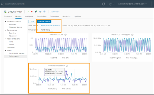
Figure C-2. Identifying the VMDK of the VM experiencing the most latency
This view also allows us to determine the physical disk placement, or in other words, which hosts are housing the VMDKs associated with the VM. Figure C-3 shows that the replica objects for "Hard disk 2" is located on ESX01, and ESX02. We will want to identify which is the primary host contributing to that latency, which can be achieve through the host level metrics.

Figure C-3. Identifying the host location where the VMDK object resides.
Step B: View metrics at the cluster level to provide context and look for any other anomalies.
Before we go to the host level metrics, it is important to gain context of the activity across the entire cluster. This will help us identify if there was some other activity that changed that may have impacted vSAN’s resources across the entire cluster. This is a great way to see if the issue is an anomaly, or systemic. Figure C-4 shows that there was indeed a latency spike in reads across the cluster.

Figure C-4. Reviewing activity at cluster level to provide context to conditions
We can also verify what type of latency is being identified. Figure C-5 indicates that it was read latency, and not resynchronization read latencies. We can also see in this view that there were no congestions during this displayed time window.

Figure C-5. Reviewing "Backend" graphs to determine the type of read latency
Step C: View metrics on host to isolate type of storage I/O associated with identified latency.
We will want to select one of the two hosts indicated above that is showing the most latency under the VM tab. As Figure C-6 shows, ESX02 shows this latency spike we were viewing at the VM and cluster levels.

Figure C-6. Verifying the spike in read latency on the host
By clicking on the "Backend" tab as shown on Figure C-7, we get confirmation again that this latency not coming from resynchronizations.

Figure C-7. Determining that the read latency was not coming from resynchronizations
Step D: View metrics on host, looking at host network VMkernel metrics to determine if issue is network related.
We see in Figure C-8 that the host network tab shows that no visible pack lost percentages were occurring on this host. This helps us determine that the associated read latency is not a result of dropped packets.

Figure C-8. Verifying that there is no visible level of packet loss occurring on the host
Step E: View metrics on host, looking at the disk group level to determine type and source of latency.
This can be achieved by the "Disks" tabs in the UI. By viewing the entire the "whole group" option as shown in Figure C-9, we can confirm that the read latency spike is coming from frontend traffic.

Figure C-9. Confirming read latency spike is coming from frontend traffic
Scrolling down, we can see in Figure C-10 that the "cache disk de-stage rate" had a substantial amount of destage activity at the same time the latency spike occurred. .We can also see that this destaging activity was freeing up capacity in the write butter, as the "Write Buffer Free Percentage" changed during this same period.

Figure C-10. Observing the destaging rate, and the percentage of write buffer space free
Scrolling down further, we see in Figure C-11 that there is no indication of congestions occurring on the disk group, and no noticeable change in the Delayed I/O percentage.

Figure C-11. Verifying that there are no congestions
Scrolling down to the bottom of this view, we see in Figure C-12 that there is no correlation in delayed IOPS or throughput that correlate with this latency spike. This indicates that the queue used for frontend VM traffic is in good shape and capable of accepting more I/Os into the queue.

Figure C-12. Viewing Delayed I/O and associated latency activity of disk group
If we change the view to show the NVMe buffer device as shown in Figure C-13, we see that The buffer device shows a burst in read IOPS and throughput reflecting the destaging activity previously identified. Note here that there is no change in read or write latency at the buffer, indicating that the reads being fetched by the VM were all coming from the capacity tier.

Figure C-13. Read IOPS reflecting the buffer destaging activity, with no spike in latency
Let's change the view to show one of the two capacity devices in the disk group. On this device, as shown in Figure C-14, we see write activity representing the destaging that is occurring, but also read activity representing the reads requested by the VM. The associated latencies during this period go up, but only to a peak of 0.562ms for the physical layer latency, and 1.512ms for the vSAN layer latency.
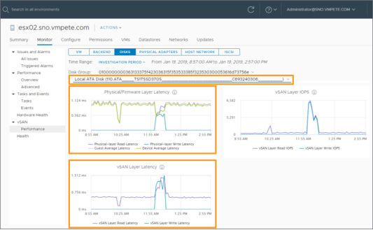
Figure C-14. Reviewing read and write latencies for the first of two capacity devices
If we change the view to show the second of two capacity devices in a disk group, we'll notice some interesting results. As shown in Figure C-15, during that same period of destaging activity, and simultaneous VM reads, we see the physical layer latency and the vSAN layer latency significantly higher than the other capacity device in the same disk group: Over 7.5x higher for physical layer latency, and over 6.9x higher for vSAN layer latency. This clearly shows one specific capacity device having abnormally high latencies compared to the other capacity device.

Figure C-15. Noticing much higher read and write latencies on the second of two capacity devices
Now let's refer to a previous HCIBench test result time window to see if this is consistent with any synthetic tests. We will check the results of the HCIBench stress test on the capacity device showing good latency values first. As Figure C-16 shows, we see physical layer latencies no higher than 1.5ms, and vSAN layer latencies no higher than 4.5ms.

Figure C-16. Checking latency on first of two capacity devices from a previous HCIBench stress test
When we view the HCIBench test result time window for the second capacity device showing questionable latencies under real workloads, we see that the synthetic tests also illustrate that there is a problem with this device. As shown in Figure C-17, we see firmware latencies as high as 11.7ms, and vSAN layer latencies over 40ms. The degree of difference In performance of this device under synthentic tests was similar to what was seen with the production workload.

Figure C-17. Noticing much higher latencies on second of two capacity devices from a previous HCIBench stress test
Step F: Come to a conclusion and course of action based on results.
Based on the test results, we can conclude that the higher than average read latencies were occurring because of one physical capacity device in the disk group was unable to commit writes (during destaging) and fetch reads (guest VM requests) concurrently in a timely manner. The primary reason for this poor latency on this device is because it was a flash device that is not on the VMware Compatibility Guide (VCG) for vSAN, due to it not meeting VMware's testing standards for performance and consistency. This is one of the reasons why the hardware discovery step is an important aspect of performance diagnostics. The primary course of action would be to replace any devices that are not on the VMware vSAN VCG.
The behavior demonstrated in this example can also occur with approved capacity devices using the SATA protocol. Unlike other offerings, SATA devices transfer data in a half-duplex mode. Thus when both reads and writes are demanded of a device at the same time, non-deterministic latencies will occur as it attempts to arbitrarily complete both reads and writes at the same time. SAS and NVMe based devices do not have this constraint, and is the reason why they sit higher up on the performance pyramid shown in Figure 7. Environments that are looking for higher levels of performance with greater levels of consistency should use at the very minimum, SAS devices at the capacity tier. The second, and optional course of action would be to evaluate if this environment should use capacity devices based on SAS or NVMe instead of SATA.